Lab 06: Advanced Overlay and Suitability Modeling
GTECH 36100 GIS Analysis
GTECH 73200 Advanced GeoInformatics
Lab: Raster Overlay and Suitability Modeler
I. Objectives
Spatial overlay is “the most important feature of any GIS”, which ”combine spatial data sets (or maps), to produce new maps that incorporate information from a diversity of sources.” (Unwin) Spatial overlay can be performed on both vector and raster data. One of the most useful applications of overlay is to produce suitability or probability maps for siting or risk studies.
As most of vector overlay has been covered in introductory GIS courses, here we focus on raster overlay and use ArcGIS Pro Suitability Modeler to produce suitability maps for siting questions.
II. Lab Tasks and Requirements
We will conduct a suitability modeling work for new nursing homes in New York City, in which we try to locate their most suitable locations. Note that our case is overly simplified and is only appropriate for learning purposes.
To find good sites for new nursing homes, we will use four criteria:
Good air quality
Close to hospitals and health services
Not close to other nursing homes
Not close to subway stations
The data on air quality (PM 2.5) is available as a raster layer from NYC Open Data. And we have point data for health facilities, which contain the types for hospitals, extended clinics, and nursing homes. The NYC subway stations are also publicly available.
Download and unzip the lab data file geodatabase. Create a new ArcGIS Pro map project for the lab. Add the three feature classes and the raster layer into the Map.
TASK 1 Generate and Process Raster Data
Generate distance raster layers for distances to hospitals, nursing homes, and subway stations using the Euclidean Distance tool. Make sure the results have a relatively high resolution and NYC extent. Remember to set the Output Coordinate Systems, which also determines the unit of the Output Cell Size. Use the entire NYC as the extent and also mask to clip the raster to the city.
Euclidean Distance tool is deprecated and will be removed in the future versions of ArcGIS Pro. Please use the Distance Accumulation tool, if Euclidean Distance is not available anymore.
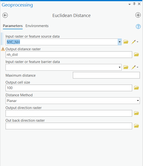
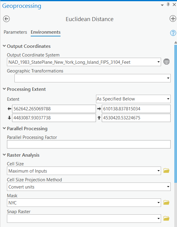
Pay attention to the Extent. Normally, we use the extent of the AOI (Area of Interest).
The following figure exemplifies the distance to existing nursing homes.
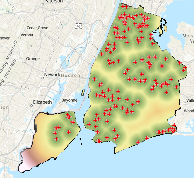
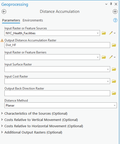
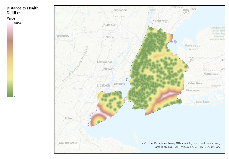
Here is the distance to Health Facilities using Distance Accumulation tool.
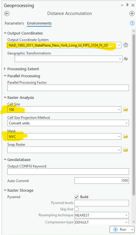
There are many options to set the “Processing Extent”. Make sure it is large enough to cover the AOI. Of course, it is always good to use the extent of AOI to set this parameter.
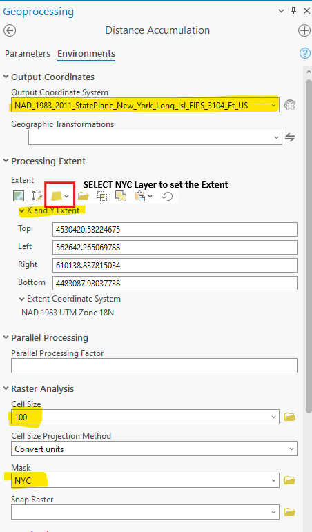
The new Distance Accumulation tool tries to optimize the algorithm’s efficiency by ignoring polygon in the mask that does not contain any point sources. In that case, the resultant raster may miss some parts of the mask, i.e., NYC in our case. If that happens to you, you can run the tool without mask and then run Clip Raster to clip the raster to the city boundary.
In the end of the task, you should have four raster layers of air quality, distances to hospitals/clinics, nursing homes, and subway stations. Next, we will derive weights for each of the four factors so that we can combine them to form a suitability map.
TASK 2 Produce Weights using AHP
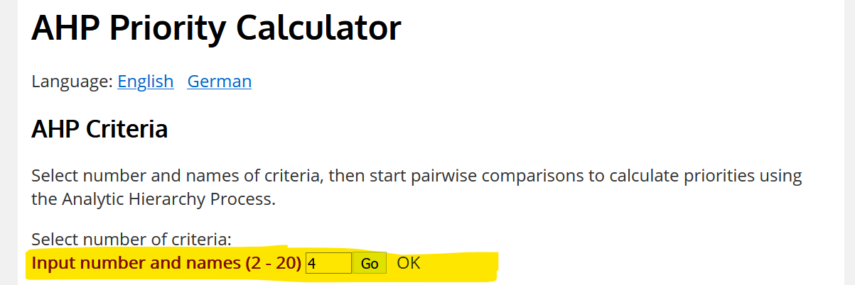
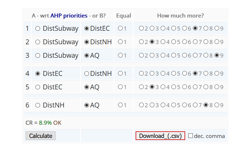
Use the online AHP calculator at https://bpmsg.com/ahp/ahp-calc.php to create consistent weights for these four factors. Note that the APH method uses pairwise comparisons and can check the consistency among the priorities.
First, type in the number of criteria (or factors), which is 4 for our case. Then type in names for those criteria/factors so that we can identify them in the next step.
Choose the more important factor of each pair using the radio checkbox. Choose 1 or Equal if you think they are equally important. If one is more important than the other, choose how much more. Press the “Calculate” button. Check the CR (Consistency Ratio) till it says OK. Note that even though we can still get weights with a large CR. A large CR means there are inconsistencies and conflicts in the pairwise comparison. For example, it is very unreasonable to have cases like Factor A is much more important than B, Factor B is much more important than C, and C is much more important than A.
You can alter the importance of these factors according to your own preference.
From the calculated priorities, we can find the weights for each criterion/factor.
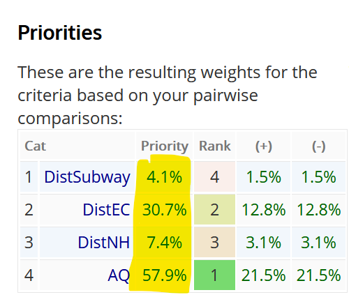
These weights (priority column) will be used in spatial overlay in Suitability Modeler.
Take screenshots to show how you have derived the weights and what they are.
TASK 3 Transform and Standardize the Raster Layers
As the criteria may have different meanings with incompatible units, it is problematic to add them together. For example, it does not make sense to add PM 2.5 and distance to hospitals. Similarly, it is misleading to directly add a distance raster layer in meter to a distance raster layer in feet. As such, we must transform and standardize the raster layer values, normally to 0 – 1 or 0 -100, etc. Once they are standardized, those criteria will be in relative scales and then can be summed and compared.
There are two goals for the transformation and standardization. First is to rescale all the raster values to the same range, either 0-1 or 0-100. Second is to make higher values favorable and low values unfavorable. For example, higher distances to hospitals are unfavorable, we need to reverse the values, that is to make higher distances lower values and lower distances higher values.
There are two routes that we can do such transformation and standardization. One is manual operation using Raster Calculator. The other is more advanced using the Suitability Modeler.
Method 1 Map Algebra with Raster Calculator
For manual operation, we only use a simple linear transformation and make the least favorable zero and most favorable one. For criteria that do not need inversion, we use:
\[x^{'} = \frac{x - min(x)}{\max(x) - min(x)}\]
For criteria that need inversion, we use:
\[x^{'} = 1 - \frac{x - min(x)}{\max(x) - min(x)} = \frac{\max(x) - x}{\max(x) - min(x)}\]
For the inversion, you can use either of two formula.
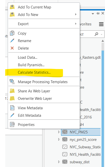
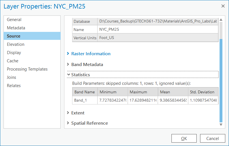
In ArcGIS Pro, we first need to “Calculate Statistics” of the raster layer. Then from layer properties, we can find the min and max values of the raster layer.
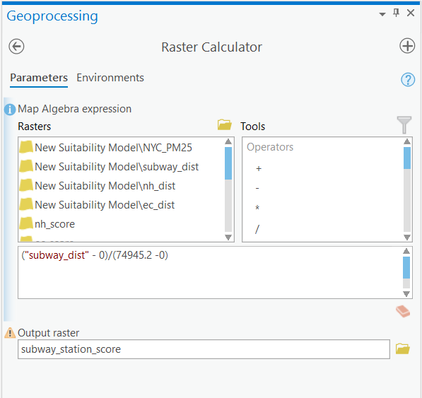
Next, we can easily transform the new values using Raster Calculator. Make sure the resultant layers have a range of [0, 1]. It is OK if the range is little bit off due to rounding. Also the higher values must be for favorable locations and lower values are for unfavorable locations.
The following are two examples with and without inversion.
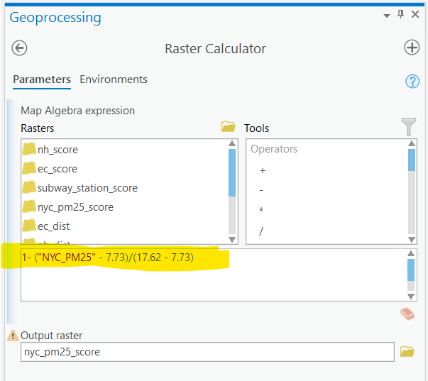
Take screenshots to show the four transformed and standardized raster layers (show the Table of Content so that it is easy to read the value ranges).
Method 2 Suitability Modeler
The Suitability Modeler provides a more complex tool to conduct the transformation.
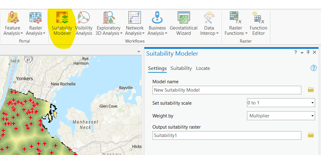
From the Analysis menu, you can launch the Suitability Modeler.
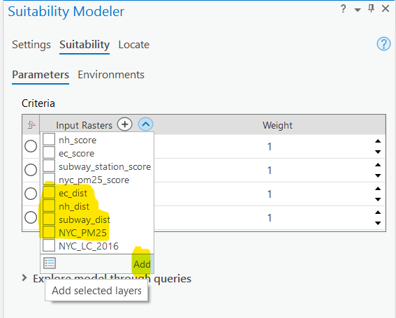
Select and add those four layers (the ones before the transformation and standardization). If your raster layer is not there, use the “+” to add Input_Rasters.
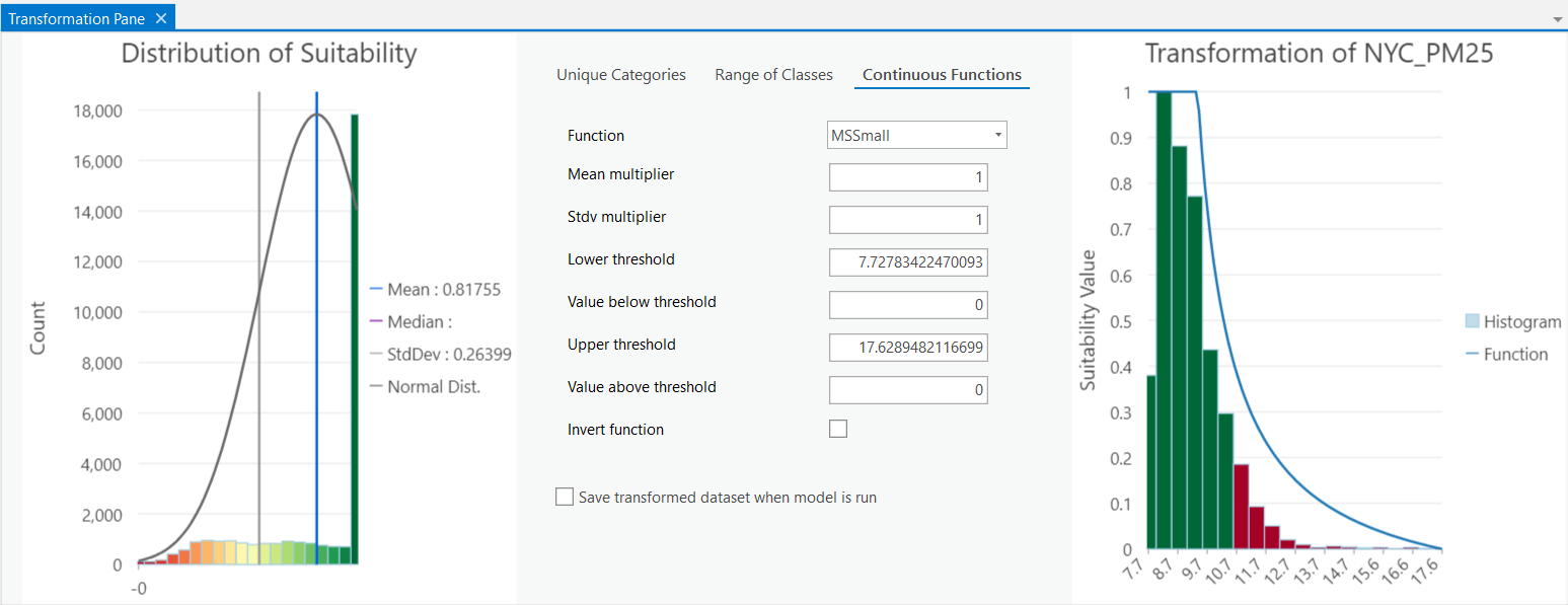
Click on the round button on the left side of the layer, we will see the Transformation Pane. By default, ArcGIS Pro would choose an “optimal” transformation that best fits the data distribution such as in the following figure.
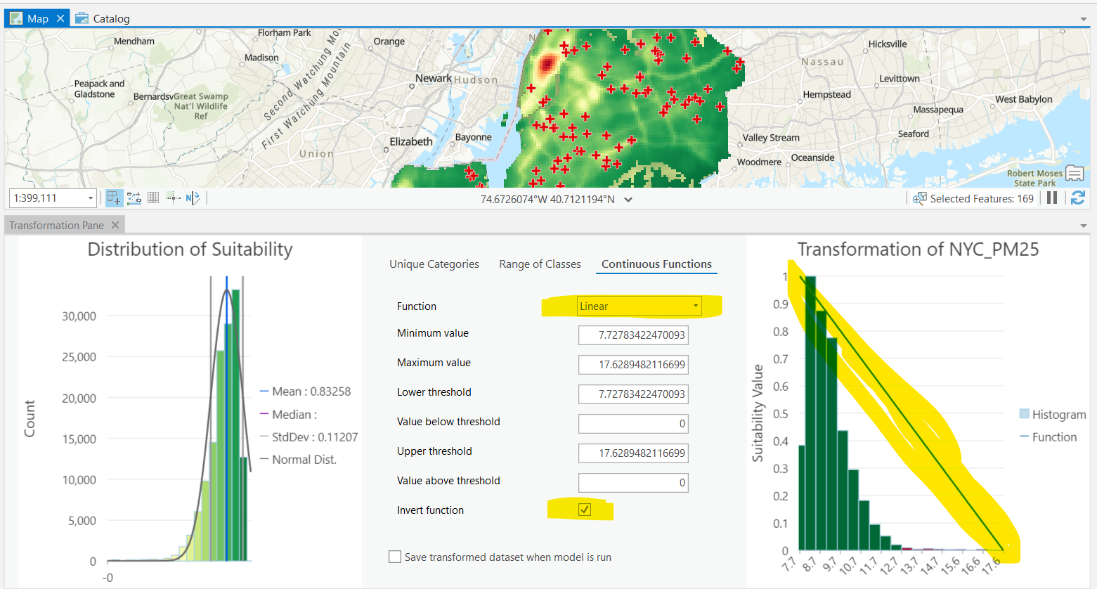
But the default one does not know that the values must be inverted for some layers. And to keep the consistency with the manual method above, we still use linear function with Invert Function checked on for the layers of PM 2.5 and Distance to Exisiting Nursing Homes. You can see from the right side that the maximum PM 2.5 values are zero, meaning least favorable. The minimum PM 2.5 values are one, meaning most favorable. The map also verifies that.
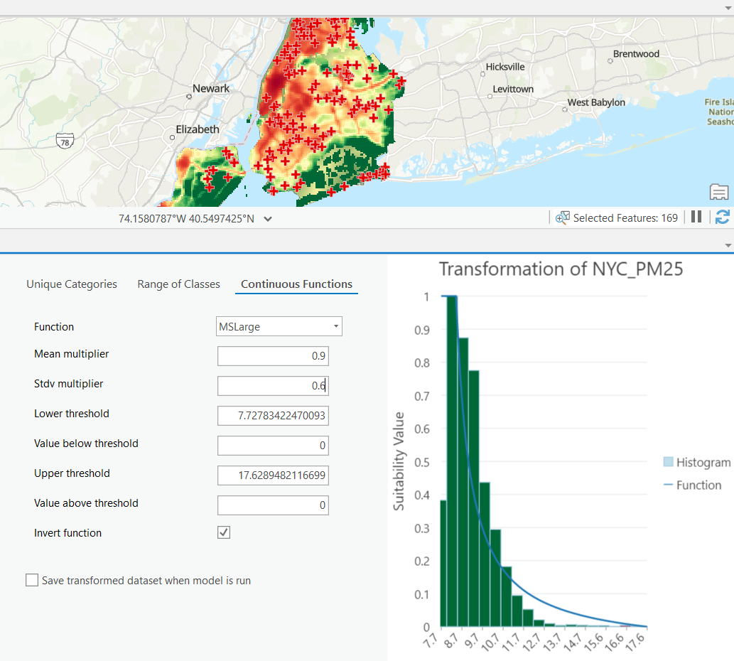
Of course, we can also use non-linear transformation functions to get a better fit. For example, we can choose MSLarge and adjust mean and standard deviation multipliers to fit the curve. Better fitted functions will create more evenly distributed values in the transformed raster layer, which however does not guarantee better results for the final suitability map.
Similarly, you can transform other layers. Overall, make sure properly set the “Invert Function” so that the high values in the transformed layer are favorable properties. For the layers that have been manually transformed, we can choose the linear transformation function without invert, which will essentially keep everything unchanged.
Take screenshots of the Transformation Pane with proper parameters for those four layers.
Task 4 Produce the Final Suitability Map
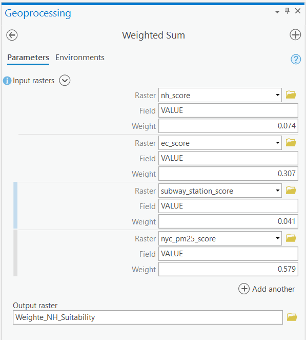
First of all, we can use tools like Raster Calculator and Weighted Sum to get the suitability maps. The weights used here are those from the AHP calculator.
With classified symbology, we can identify suitable locations for new nursing homes.
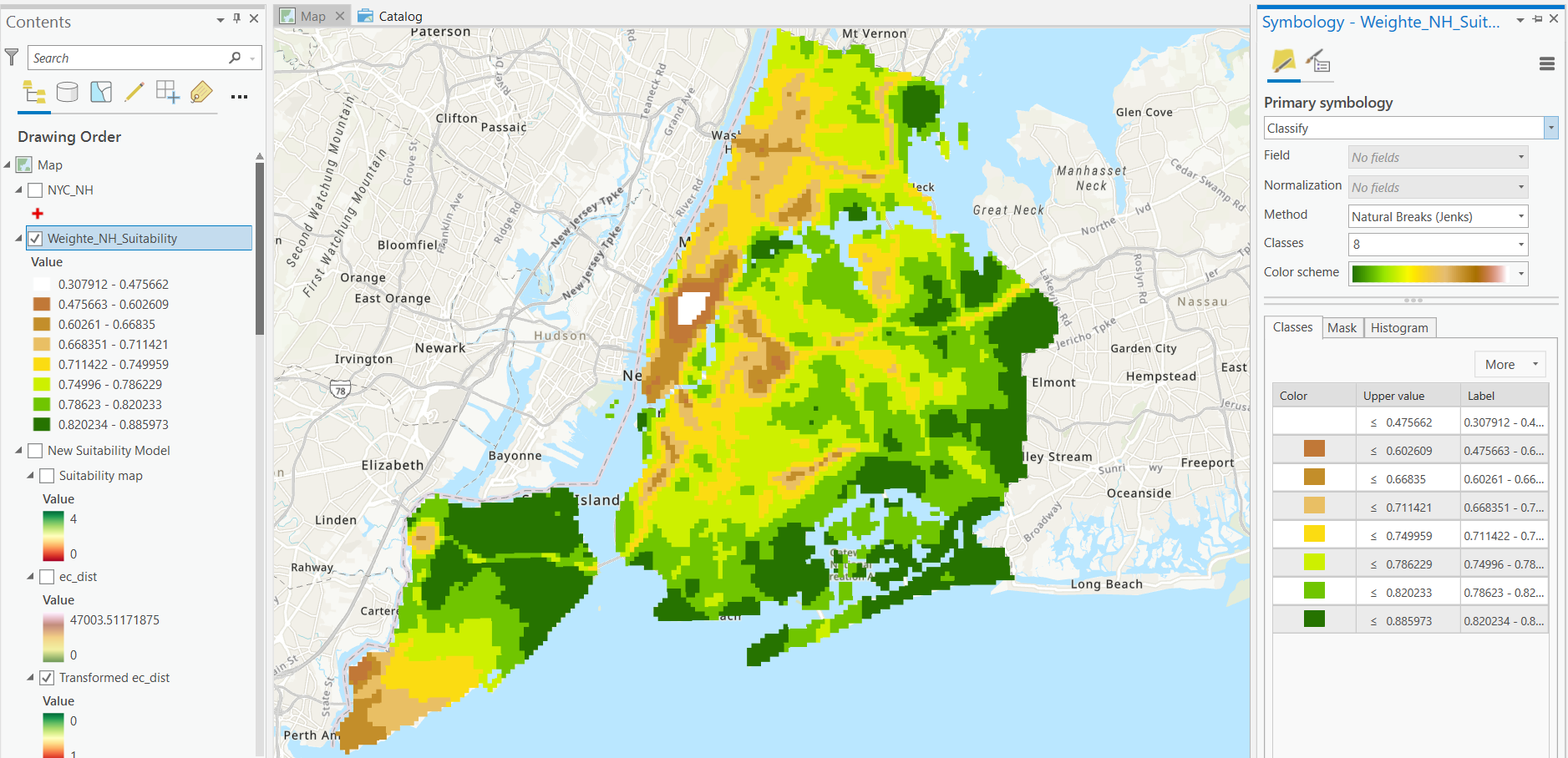
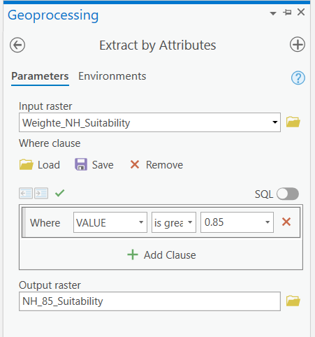
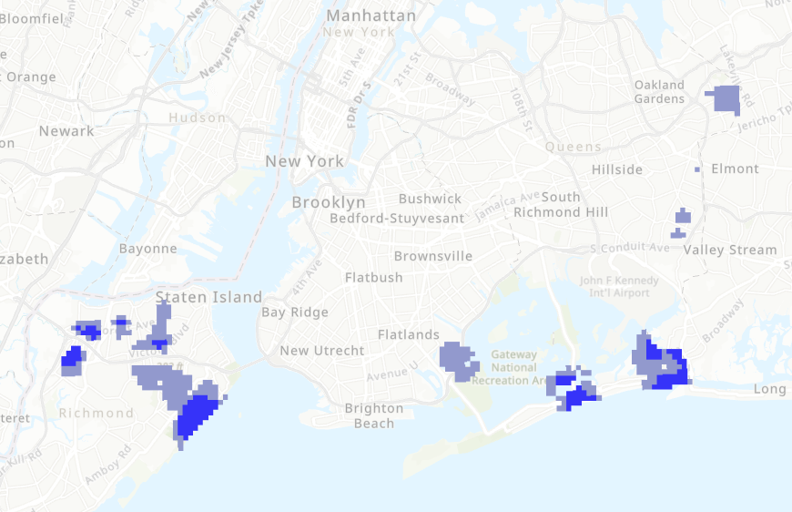
We can also extract the areas that have very high suitability values, such as > 0.85, using “Extract by Attributes” tool. And we can also convert these raster areas to vector polygons using raster conversion tools in ArcGIS Pro.
Similarly, we can use Suitability Modeler to get the results. Note that the following example used linear transformations. It also used percentage instead of multiplier in the settings.
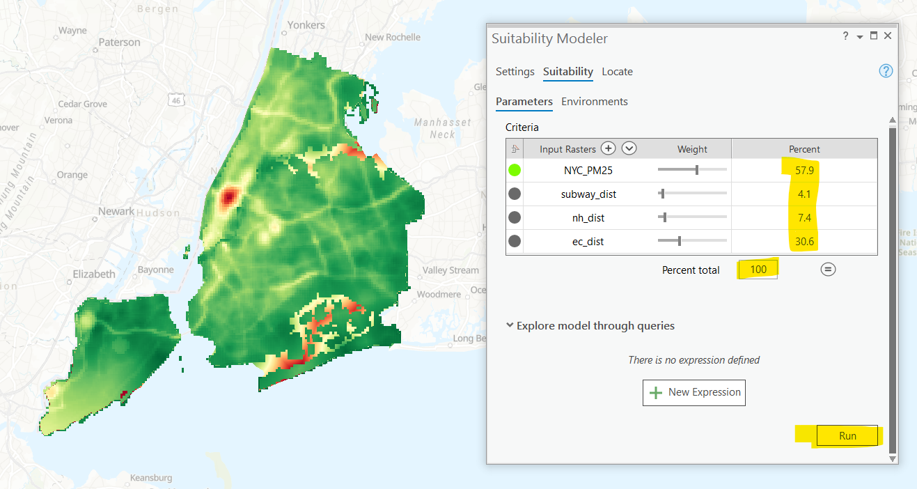
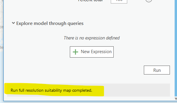
Then Run the model. Make sure you see the message “Run full resolution suitability map completed.”
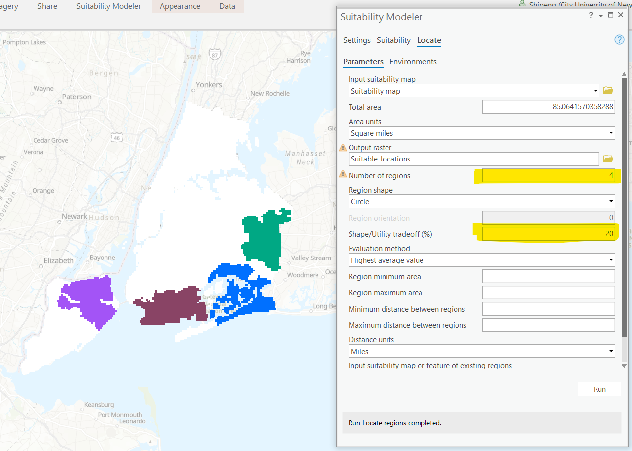
While we can use the “Extract by Attributes” tool to locate the best locations, Suitability Modeler offers a separate “Locate” tool for this task. The Locate tool takes contiguity and suitability scores into consideration and try to locate a large area with high scores. For the highly segmented urban space, it is not really applicable. Nevertheless, the Locate tool offers a simple method to identify good locations based on the suitability map.
The Locate tool identified four (we specified that number in the parameters) suitable regions. You can see that the results have a lot of similarly with the earlier results using weighted sum tool. However, these regions are mostly contiguous other than the area with isolated “islands”. These regions have the highest average suitability score as we set in the parameters.
Note that Suitability Modeler is a relatively new tool and has some stability issues. Please save your project frequently during the process.
Take screenshots of the key intermediate results.
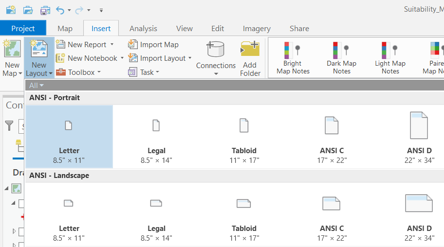
Also create a well-designed layout for the final map showing candidate locations. Most of you have already learned how to use Layout and how to add map elements like titles, legend, scale bar, graticule, etc. to the layout. If you did not learn these in Introductory GIS course, please visit https://pro.arcgis.com/en/pro-app/latest/help/layouts/layouts-in-arcgis-pro.htm for the details.
III. Instructions and Tips
The assignment must be typed and prepared in word-processing software, as hand-written work will not be accepted. The assignment answer file must be submitted through CUNY/Hunter Blackboard (bb.hunter.cuny.edu). Do NOT zip your document, do NOT send email to submit answers, and do NOT submit your data unless being asked to do so. If you have trouble using Blackboard, please contact the Hunter Help Desk.
The following file naming rule is used for this assignment when you submit the answers.
GTECH_732_361_L06_CUNY_ID.doc|docx|txt
L06 means lab 06. Do not omit the zero in the; otherwise, there would be file ordering problems on my end. Change the CUNY_ID (the [FirstName].[LastName][two digits]) to your owns.
Thank you!