Lab 05: 3D Vis and Interpolation
GTECH 36100 GIS Analysis
GTECH 73200 Advanced GeoInformatics
Lab: Spatial Interpolation and 3D Visualization
I. Objectives
For these two weeks, we learn 3D visualization and spatial interpolation, two closely related approaches for 3D data generation and analysis. From a limited number of points or other types of observations, we can create surfaces with complete coverage for an area using spatial interpolation. We can use a raster dataset or a TIN to represent the surface and render the surface in 3D, although the data are really “2.5D.” Of course, we can also use true 3D data in GIS, where Z is an independent dimension, not an attribute. 3D GIS have numerous applications in the real world and help improve the quality of geovisualization if used properly.
II. Lab Tasks and Requirements
The general process of 3D visualization using ArcGIS Pro Global or Local Scene includes a few key steps:
Generate elevation surfaces, mostly in a TIN or raster format
Apply one surface as the elevation for a 2D layer (or drape a 2D layer or a surface)
Set the appearance of 3D layers
We will use a few different exercises to learn all these methods as well as 3D analysis and spatial interpolation. But first, we need to get ourselves familiar with the 3D tools in ArcGIS Pro.
TASK 1 Use ArcGIS Pro Local Scene for 3D Visualization
Here we use a relatively simple case to learn the Local Scene in ArcGIS Pro for 3D visualization. Download a zipped file geodatabase (FGDB) that contains the water body, curbs, roadbeds, and building footprints around Central Park and Hunter College. These are clipped from the NYC Planimetric dataset.
Once again, after unzipping the file, make sure the .gdb folder is not directly within another .gdb folder. In general, a directory structure like C:\Users\Doe\GIS\data.gdb\data.gdb\ would confuse ArcGIS Pro and may cause problems for many geoprocessing tools.
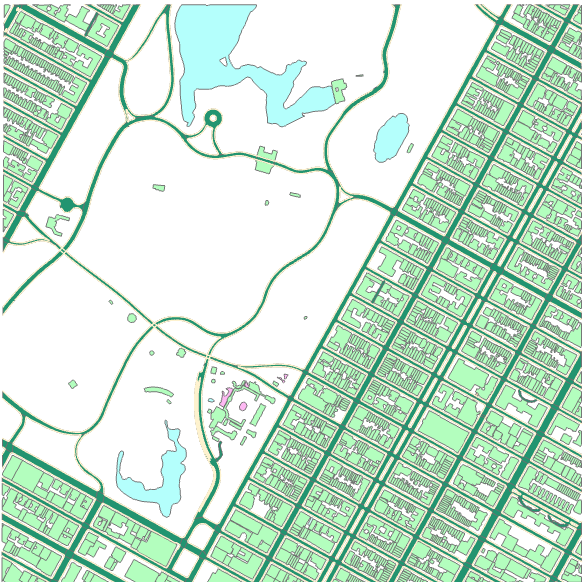
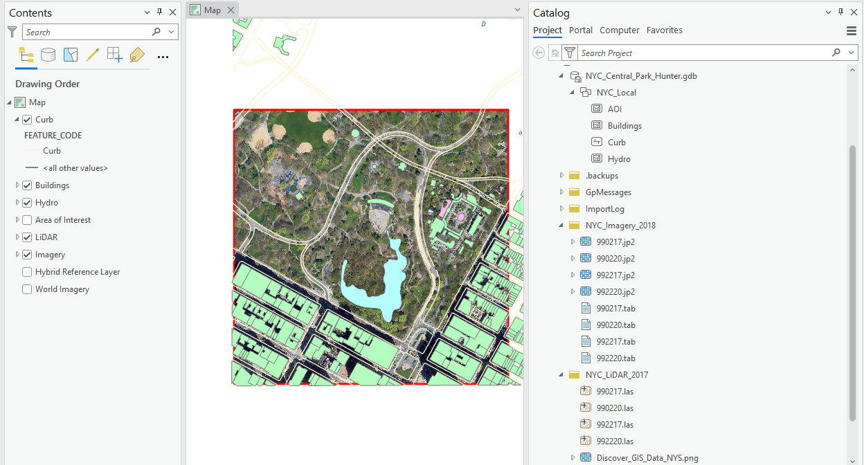
Create a new ArcGIS Pro map project. Add all the feature classes from the FGDB to the map, which should look like this.
Now we will use primarily the building footprint feature class to create a 3D visualization. In ArcGIS Pro, all 3D visualizations are performed using a special type of map: scene. As we are focusing on a small part of the NYC, we will use the “Local Scene.”
Switch to the new local scene. By default, ArcGIS Pro creates a few feature datasets and groups like 3D Layers, 2D Layers, and Elevation Surfaces. In most cases, vector layers will be treated as 3D Layers, raster images are 2D Layers, TIN and DEM can work as elevation surfaces. ESRI also add a cloud-based surface (World Elevation 3D/Terrain 3D) and 2D layers of World Topographic and Hillshade, which are like the basemaps in regular Maps.
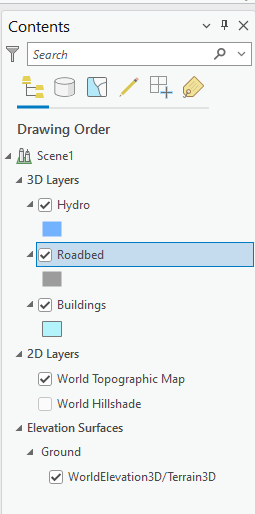
Add roadbed, hydro, and buildings to the scene’s 3D Layers. You can drag them to 3D Layers or right click each of them in Catalog and choose “Add to the Current Map”. Your table of content should look like this.
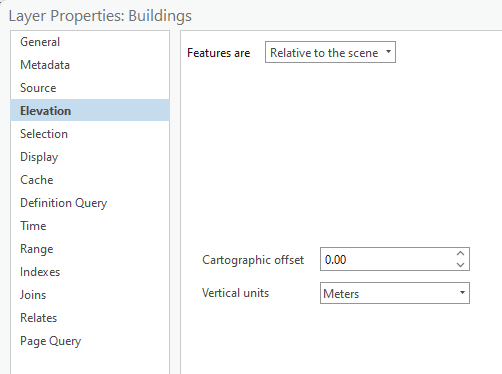
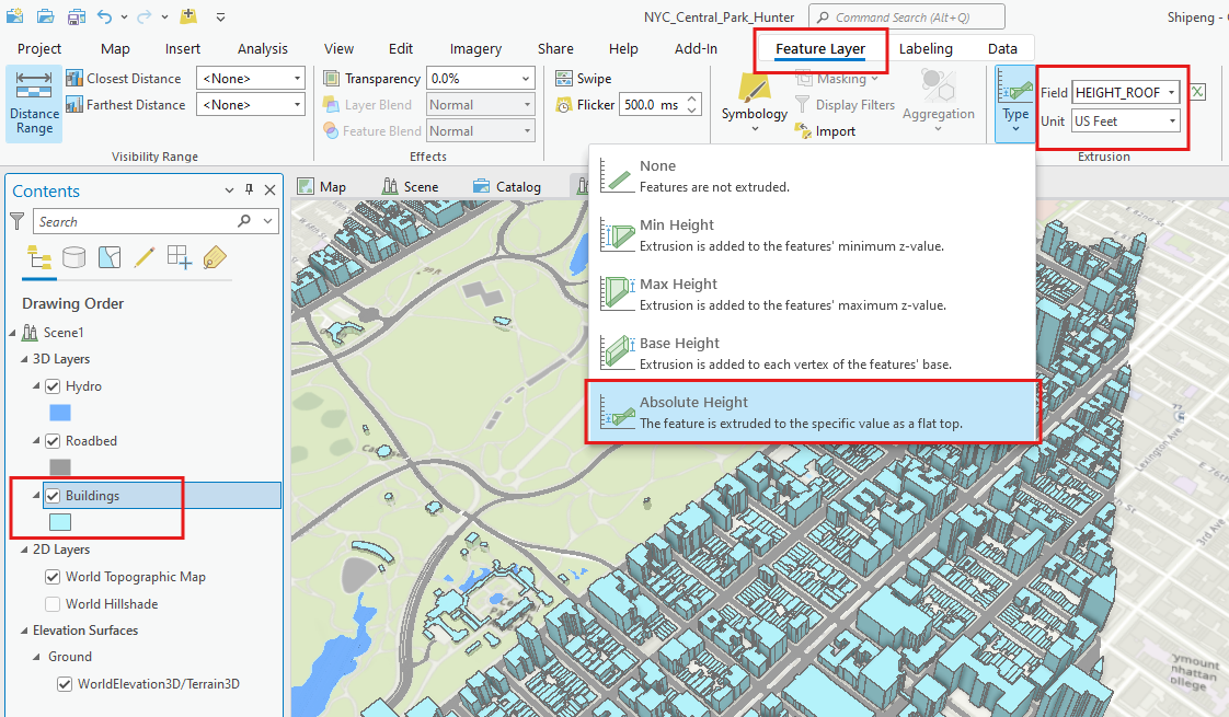
From the Layer Properties of the buildings (Right click on the layer in List/Table of Content, you can open Layer Properties), set Elevation to “Relative to the scene.” This means the height of the building that we will use later is not absolute elevation, but relative to the surface/ground.
Set the extrusion of the buildings as “Absolute Height” because this particular feature class has a field named HEIGHT_ROOF, which is the building height. The extrusion will make the building a 3D object by extruding the 2D polygon to that specific height.
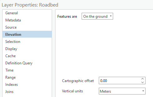
The hydro and roadbed feature classes do not have height or elevation information. So, we just make them follow the groud elevation, which is from the WorldElevation3D/Terrain3D layer in the Elevation Surfaces. Note that the “Ground” in Elevation Surfaces is WorldElevation3D/Terrain3D.
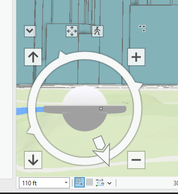
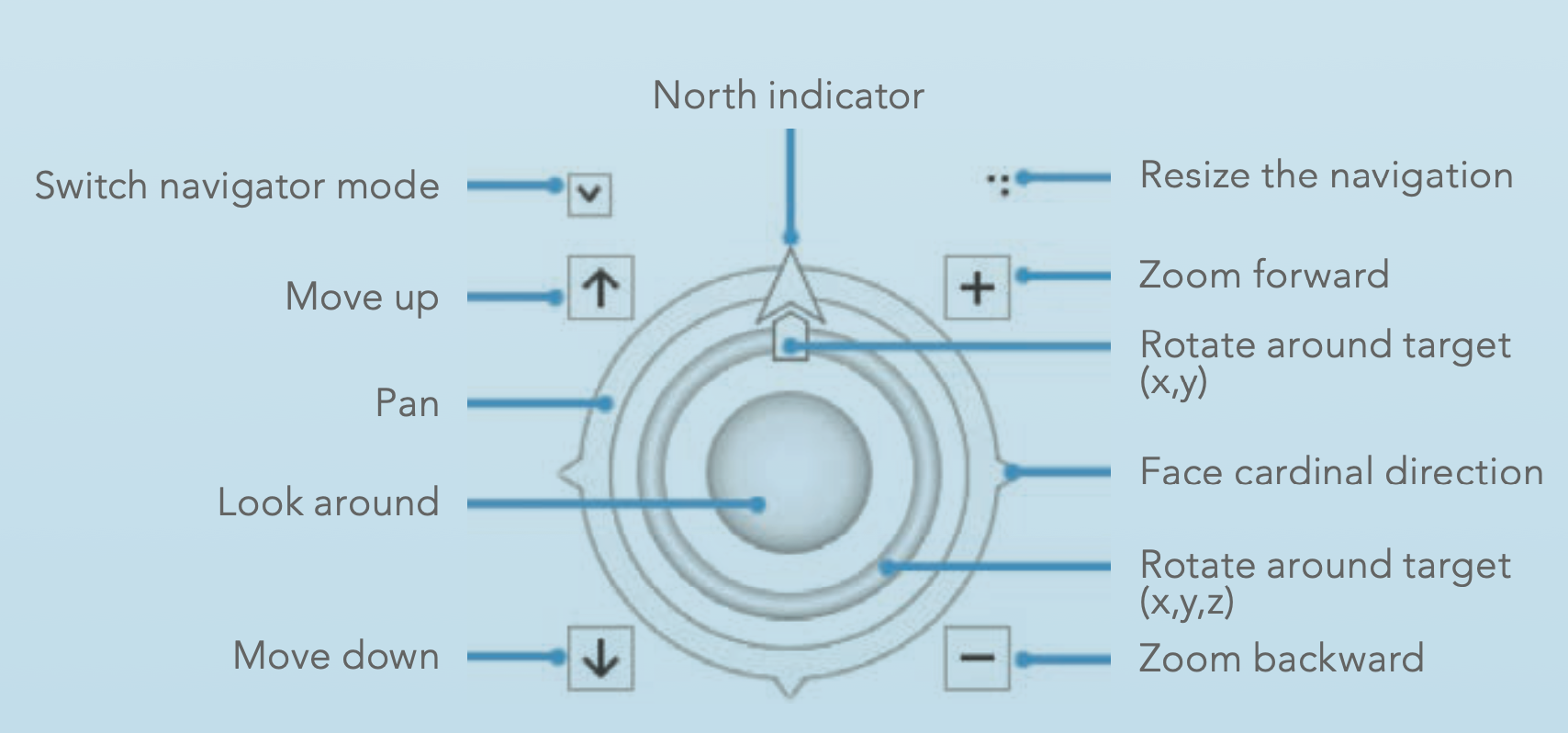
As such, we have a very simple 3D visualization of these feature classes. Now, use the Navigation tool to move around the “3D” view. Unlike the 2D navigation, 3D navigation sometimes is not very intuitive. Please read General 3D Navigation in ArcGIS Pro, particularly the On-Screen Navigator as pictured below.
Use the on-screen navigation tool and/or keyboard, customize the local scene view to show the two skybridges over Lexington Ave and 68th Street. In addition, the symbology of all these vector features can be configured in a similar fashion as in 2D Map.
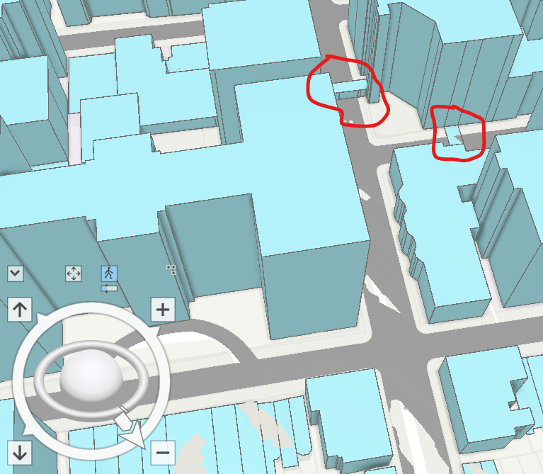
Take a screenshot of your view showing the two skybridges. Change the colors of the buildings and edges to different colors or patterns.
TASK 2 Build TIN dataset using LiDAR
From TASK 1, the ground surface is quite important for 3D visualization, particularly for environmental applications with natural phenomena. Here we will learn how to create elevation surface using LiDAR.
One important data format for elevation surfaces is Triangulated Irregular Network (TIN), where the elevations at triangle vertices are known and elevation at other places can be interpolated simply using the triangles. Today, the most common approach of acquiring elevations at sampled locations is LiDAR (Light Detection and Ranging). The details of LiDAR technology and data processing are covered in our Remote Sensing classes. Here we only learn how to use LiDAR data to generate TIN in ArcGIS Pro.
STEP 1 Find and Download LiDAR and relevant data
In the United States of American, most, if not all, states have LiDAR data publicly available. The State of New York collected LiDAR data for multiple years and the entire state is covered. We only use a small area in Central Park near Hunter College for learning. You are free to explore and utilize LiDAR from other areas for the assignment, particularly if your final course project might use LiDAR as well.
Search and go to DISCOVER GIS DATA NY website at https://orthos.dhses.ny.gov/. Open the left panel (Click on the right arrow). Pan and Zoom to the area of your interest.
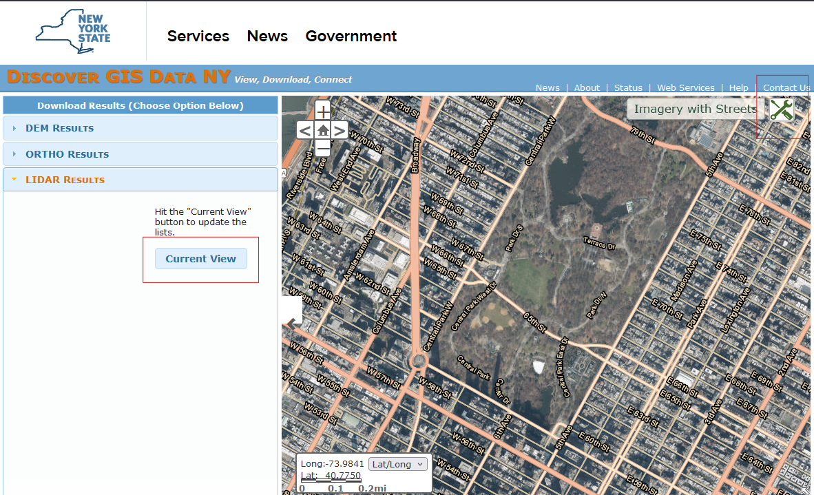
Click on “Current View”. We will see the available LiDAR data in the mapped area. You can also use “Settings” on the top-right corner, then “Layer Control” to set the visibility of map layers just like in a regular GIS program.
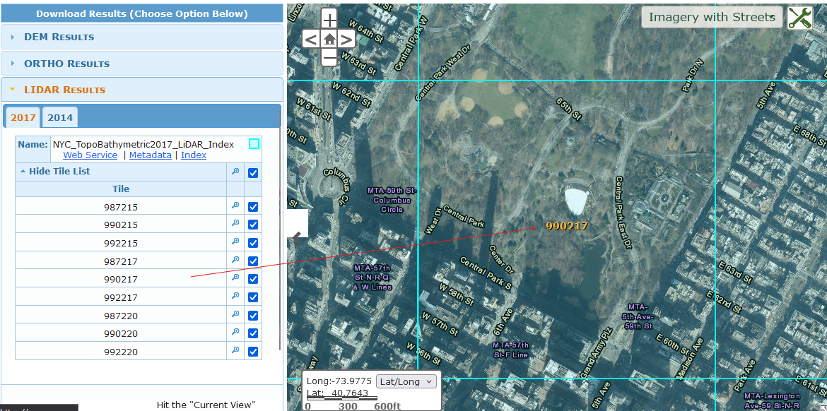
Now, you should be able to see all the data that are, wholly or partially, within the view. If there are too many results, you can further zoom in and refresh the “Current View”. As the NY 2017 LiDAR data has a very high resolution, we only try one tile with the index of 990217. Click on the tile index in the results, which will download the 990217.las file. LAS is a standard LiDAR point cloud file and is readable in ArcGIS Pro.
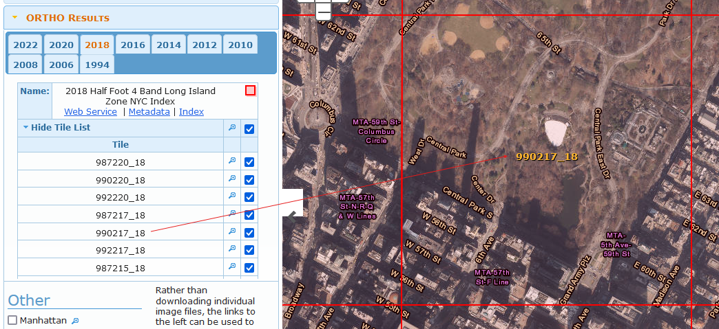
At the same time, download the orthophoto of the same tile from 2018 (in ORTHO Results, right above LIDAR Results). Both 2017 LiDAR and 2018 ortho use the same set of tiles and they align with each other very well. Download the ortho by clicking on its tile index. It should be a zip file. Unzip the file. You should see a jp2 (JPEG2000) and a few associated files.
Note that the dataset in TASK 1 FGDB contains four tiles in total, not only for the tile 990217, just in case you want to try a different tile on your own.
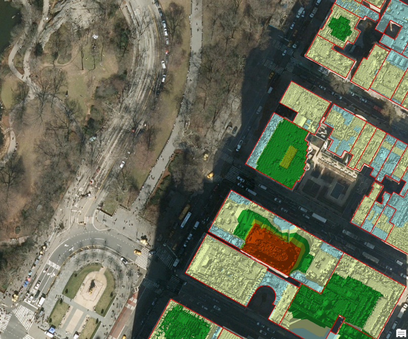
Add all data into an ArcGIS Pro map project. Ideally, all the vector data should be a feature dataset with a local projection/spatial reference system (State Plane Long Island). It should look like the following screenshot.
Step 2 Create TIN data
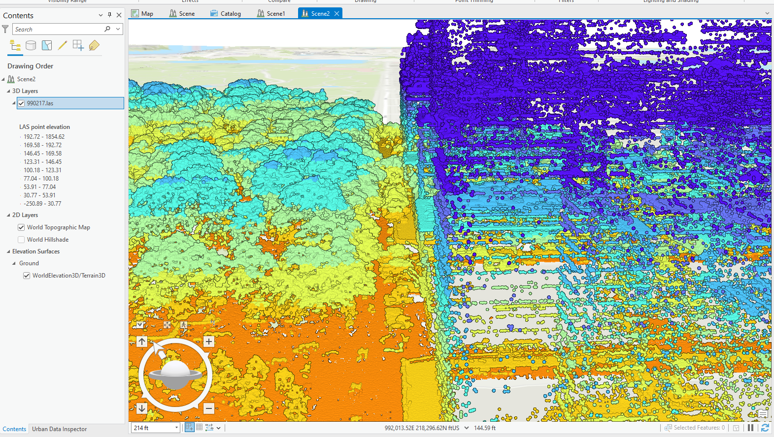
As LiDAR is such an important and popular data source for elevation surfaces, ArcGIS Pro offers a “LAS Dataset to TIN” geoprocessing tool, which can directly create TIN from LiDAR data. One important parameter in this tool is thinning. When we zoom in on the LAS dataset, we can see that the data density or resolution is very high. This data cloud has been used to construct objects like buildings or trees.
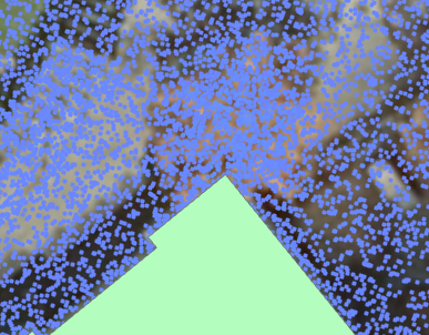
For elevation surfaces, it may not require so many points. Therefore, we can “thin” the data for a coarser surface but smaller size and faster processing. Here we just randomly choose one fourth of the LiDAR points.
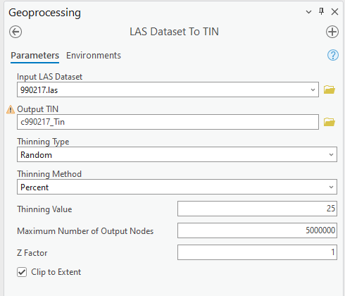
The resultant TIN still contains a lot of details. If your computer is slow and does not have a big memory, you can further reduce the percentage to 10, 5, or even 2 percent.
Step 3 Visualize 2D Ortho Photo in 3D with the TIN surface
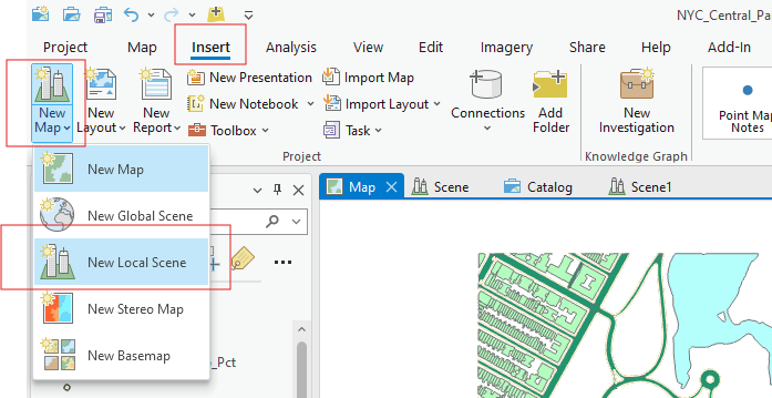
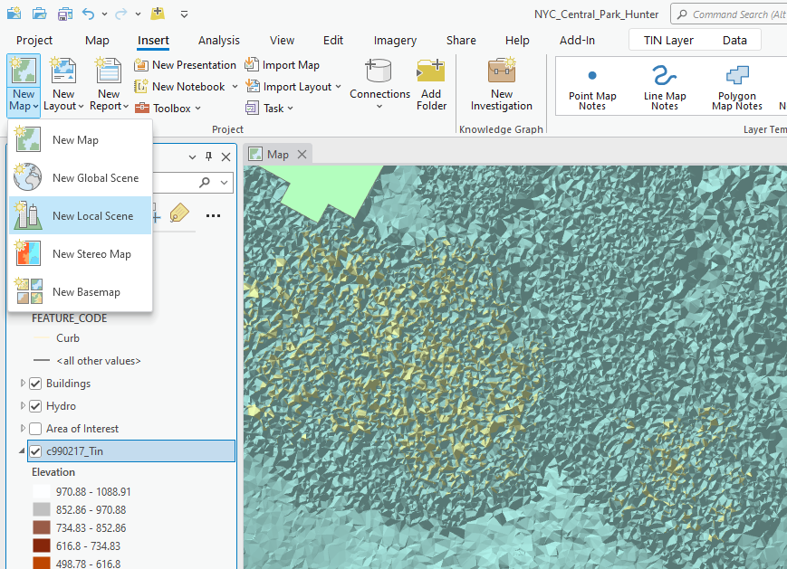
Now we can use the TIN dataset to visualize 2D data in 3D. To do that, we must use a Local Scene, which you can create from the “New Map” ribbon.
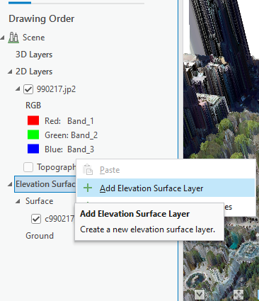
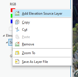
In a local map scene, we could add different elevation surfaces. First, right click on “Elevation Surfaces”, then “Add Elevation Surface Layer”. By default, this will add a “Surface” feature dataset. Now, let’s add the TIN that we created in Step 2 by right clicking on “Surface”, then “Add Elevation Source Layer”. Just browse your computer and choose the one created earlier.
Now, also add the orthophoto 990217.jp2 to the 2D Layers. You can just right click on the image in Catalog and then “Add to the Current Map”.
By default, ArcGIS Pro adds a low-resolution surface and some base maps for the local scene. But we will not use them. You can either remove them or turn them off.
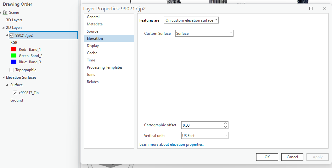
Now we can apply the surface to the image elevation property. Open the layer properties of the orthophoto. Make the “Features are on custom elevation surface” and choose “Surface” that contains our TIN.
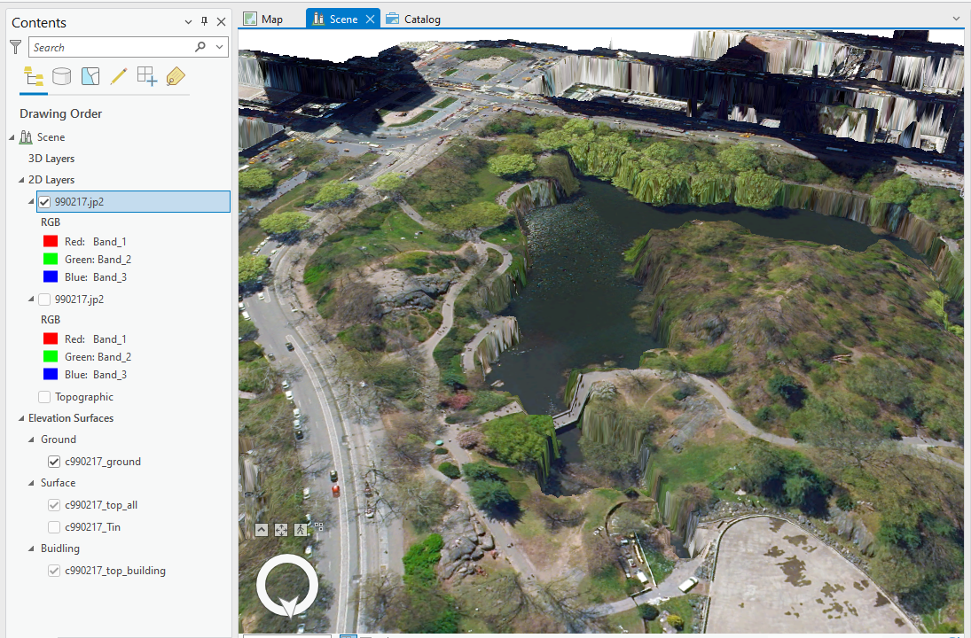
Turn off other layers. The 3D scene should like the following. Note this could take some time to render, depending on the power of the graphics card on your computer.
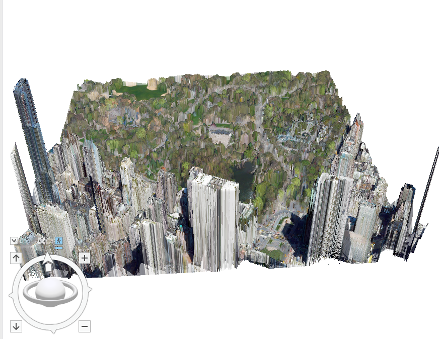
Take at least three screenshots of this scene from different perspectives, such as from north to south, near the ground, from the street, etc. This is to make sure that you 1) generated the 3D scene and 2) know how to use the 3D navigation tool.
As the city landscape is complex with buildings, roads, trees, water bodies, etc., the 2.5D surface generated from LiDAR does not look very realistic. It would work much better in the setting of natural environment.
Step 4 Ground Elevation Surface in LiDAR (Optional, 2 Bonus Points)
If we examine the principles of LiDAR, we understand LiDAR data contains multiple returns from top of the objects, buildings, vegetation (tree leaves, branches, trunks, etc.), and ground.
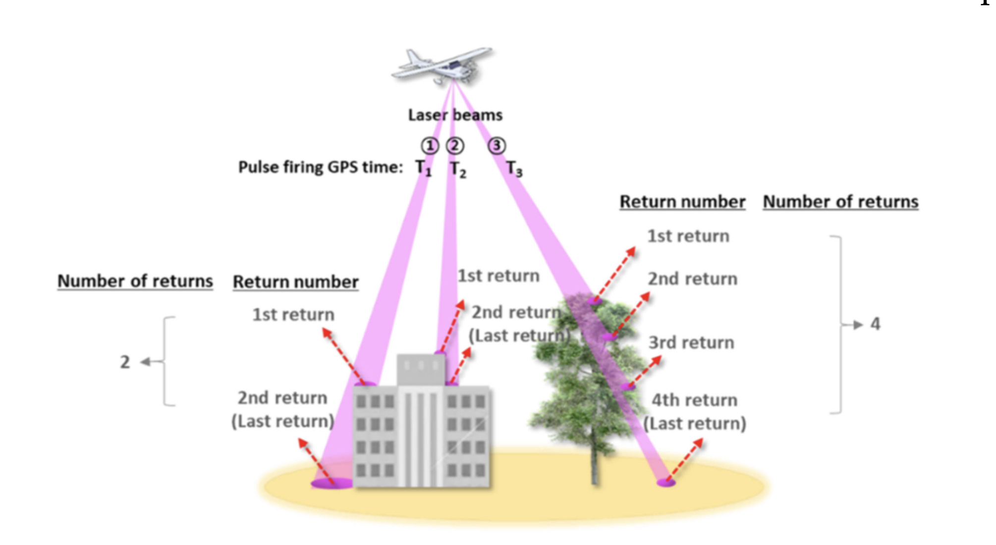
In fact, we can utilize such different returns and classification to create different surface models. If we just use the LiDAR return from the ground (bare earth), we will get the Digital Elevation Model (DEM). If we use the first return, we can get a different surface for the top of the ground objects.
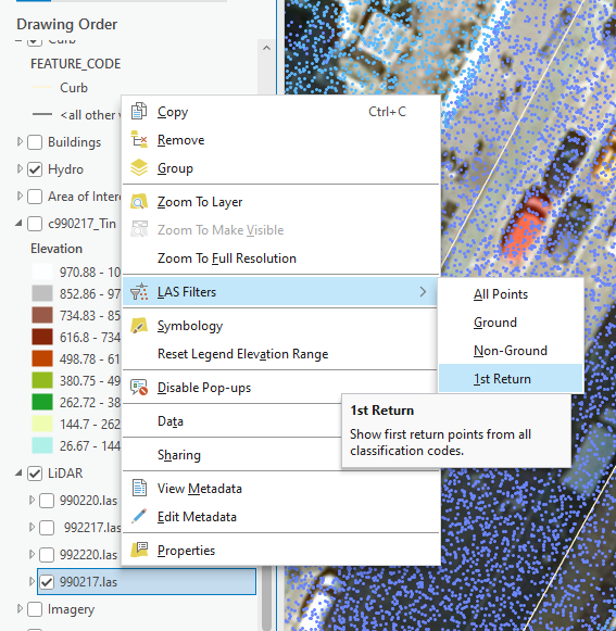
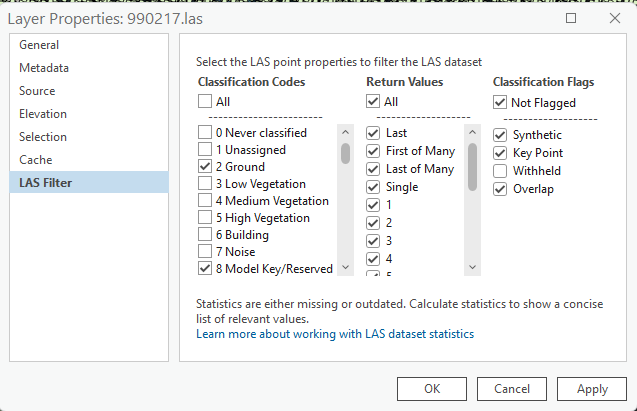
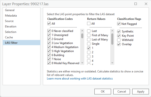
As show below, we can use Layer Properties to check out the return and classification information. The LAS filter allows us to show only a subset of all the points in the LiDAR dataset.
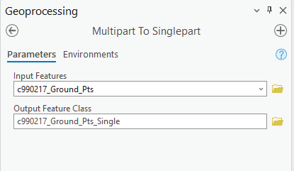
To specifically choose a class and/or return for digital surface model, we can first convert LAS to Multipoint. Then use “Multipart to Singlepart” to make them individual points. The following tool parameters use a classification code 2, which is ground. The results will only contain points returned from the ground, not trees or buildings.
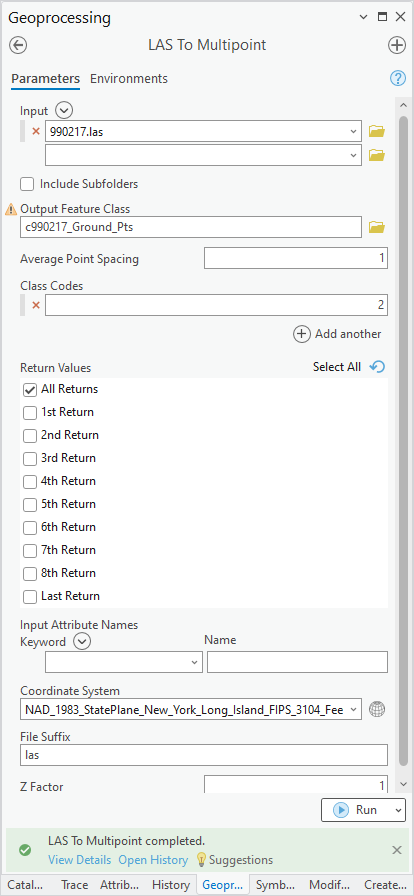
The choice of all classification codes and first turn is good for the top of objects. As we want to drape an aerial photo on the 3D surface, this setting will be best for that purpose.
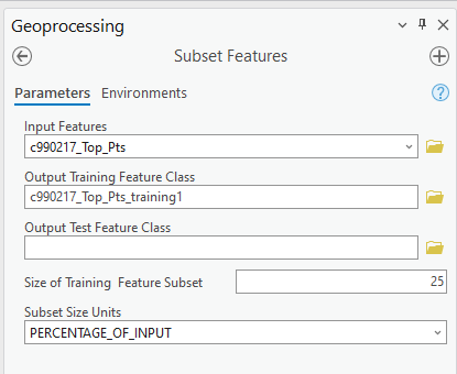
For the thinning part, we can use a tool called “Subset Features”, which can choose a specific number of results or a percentage.
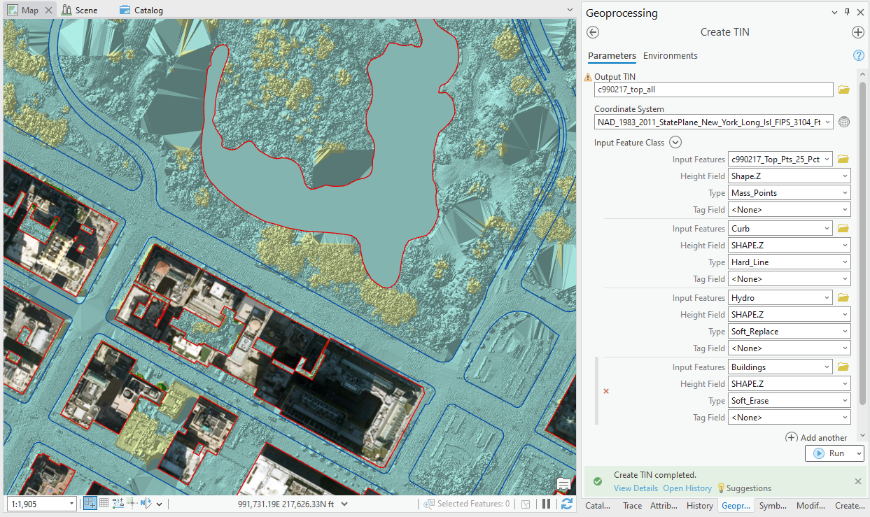
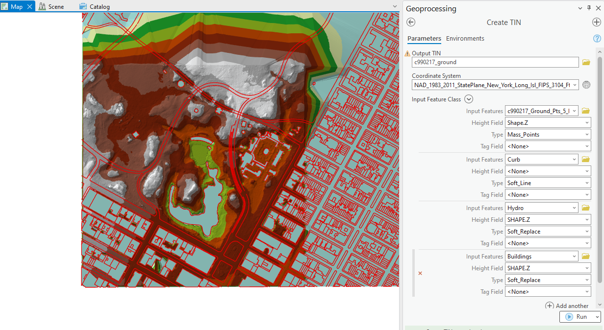
With a set of thinned LiDAR-derived points, we can use “Create TIN” to produce a surface. Unlike the “Las to TIN” tool, we have more options and control in this “Create TIN” tool. We can apply breaklines and clip zones for the TIN. Specifically for the exercise, you can try the following parameters.
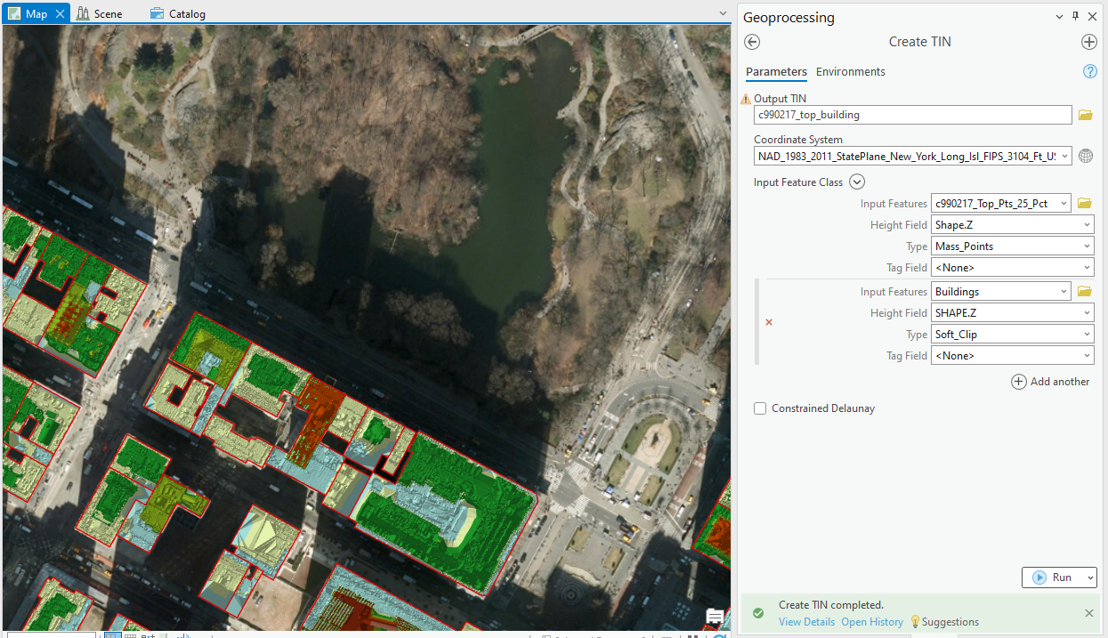
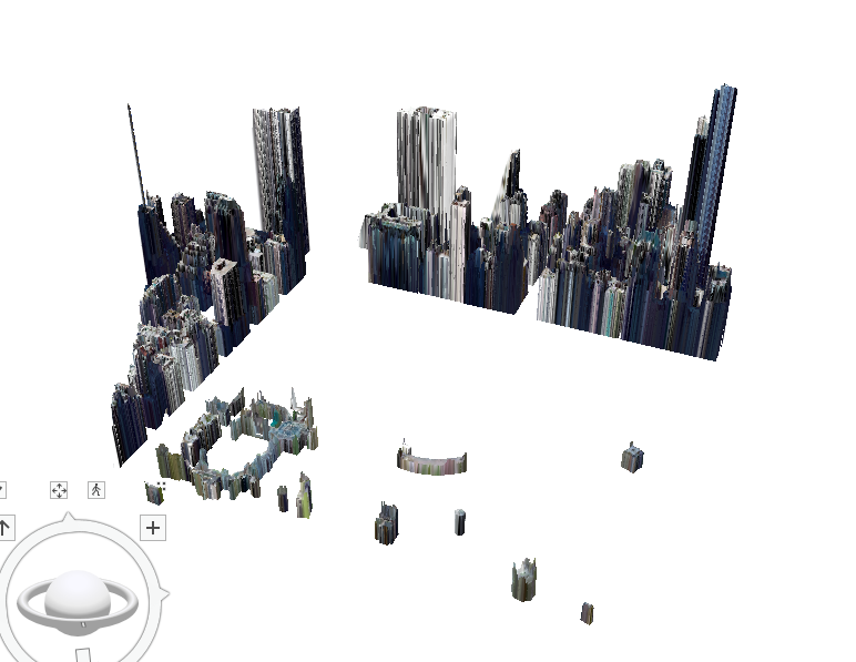
This will “clip” the surface using buildings polygons. In other words, surfaces are only kept for the buildings. As shown in TASK 1, you can drape the aerial photo on this building-only surface. The results look like the following screenshots.
If we want to keep other features, we can change the settings of the “Create TIN” tool. The following are “top” for all features.
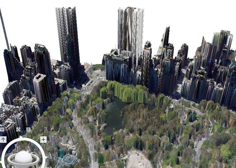
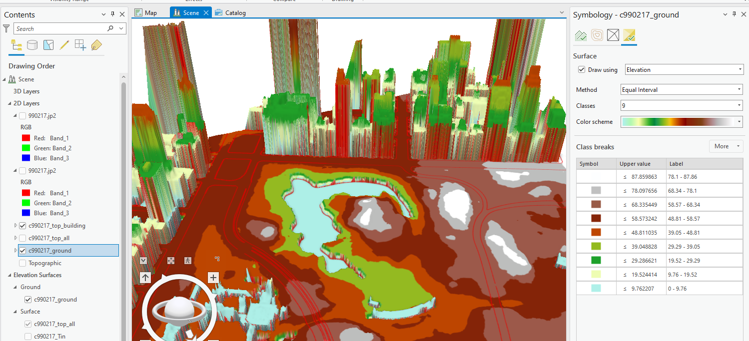
The following are for “ground” only.
Note that the TIN dataset itself can be added to the local scene and be viewed as a 3D surface.
The same is true for the LiDAR point cloud.
Take screenshots of your “Create a TIN” tool, showing parameters and success message, and a rendered local scene using your own TIN as surface.
With LiDAR data, the limitation of such “2.5D” surfaces is quite clear. If we use the “top” of objects, roads do not look good because there are tree branches and leaves over the roads. The trees are not realistic, either, because they are all “cylinders”. If we use the bare earth model, roads will look good but trees are all on the ground. In fact, LiDAR is true 3D. Reducing it to 2.5D eliminates much useful information. More advanced LiDAR tools/programs can produce real 3D objects from the point cloud.
TASK 3 3D Visualization Applications
You can choose either of the two options. Finishing both will earn you two bonus points.
Option 1: Integrating LiDAR, Extrusion, and Aerial Photos for 3D Modeling
Follow and finish the “3D modeling with ArcGIS Pro” tutorial in PDF or at ESRI Website with the accompanying data. This essentially combines the techniques in Task 1 and Task 2.
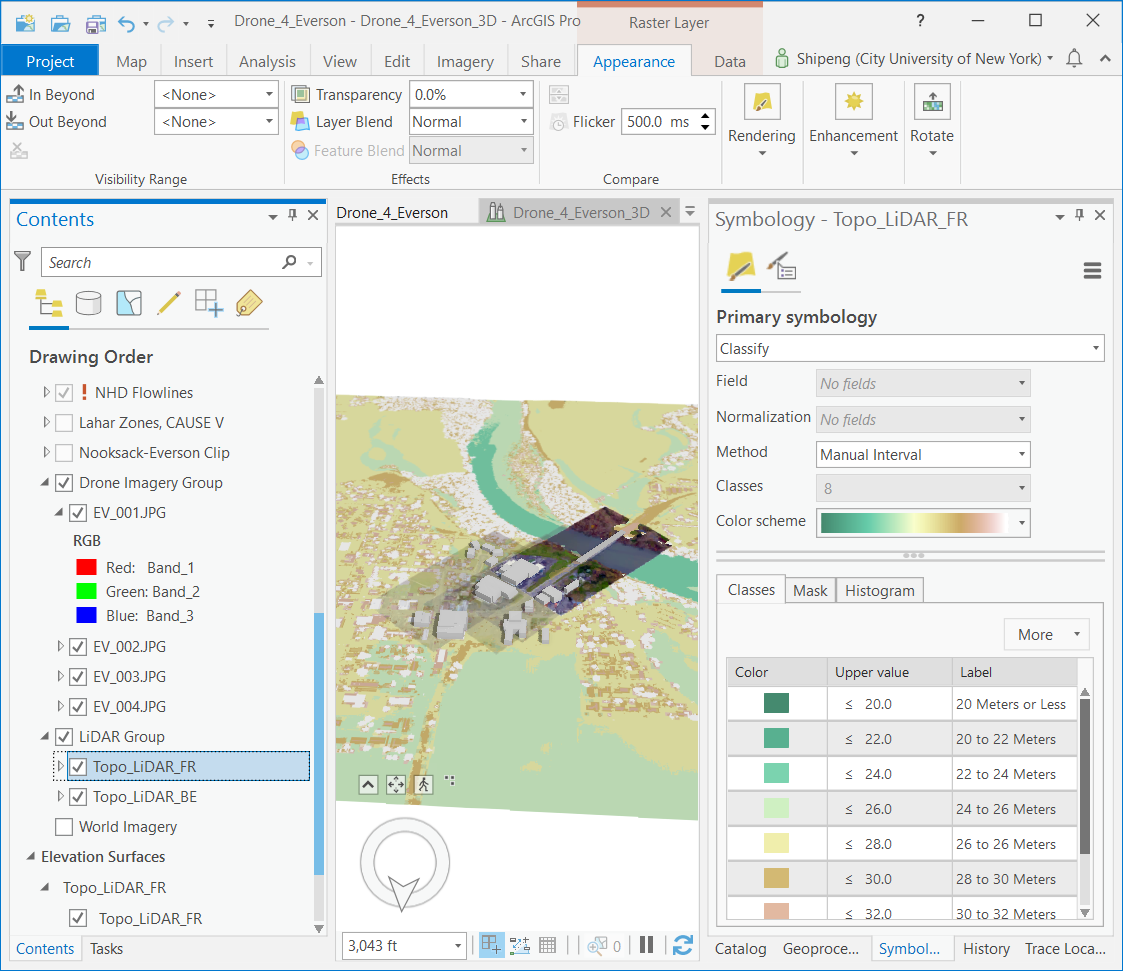
Change the layer symbology and replicate the following visual effects.
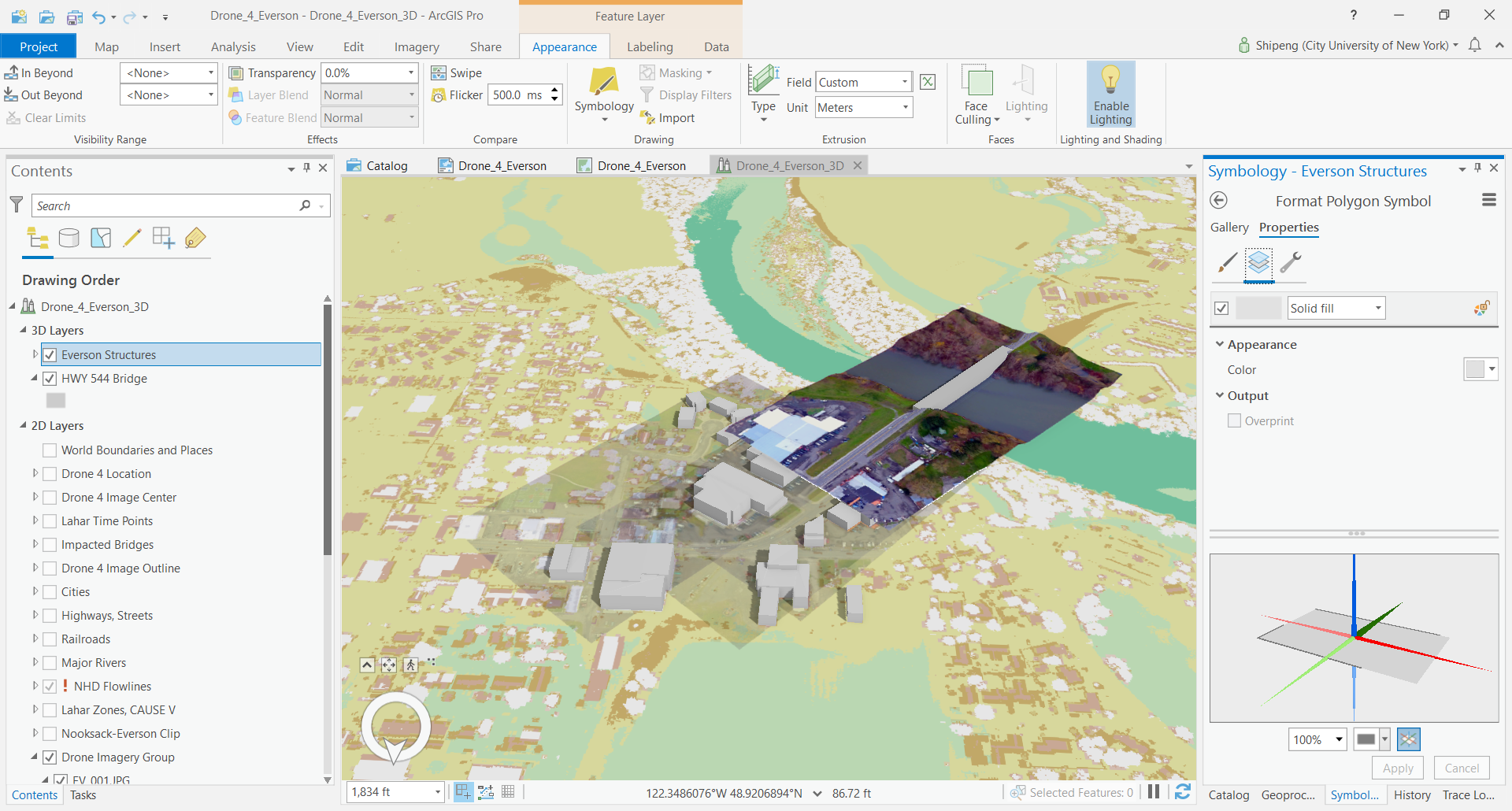
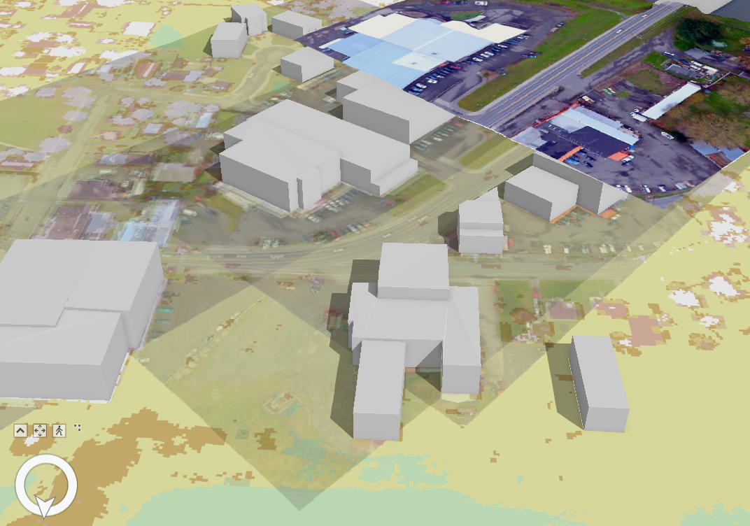
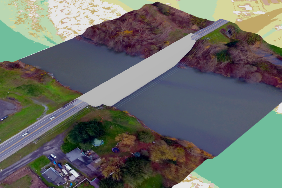
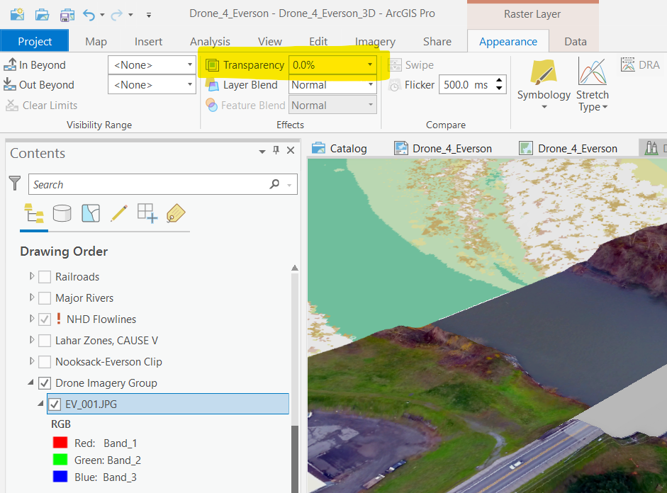
A few key settings for the layers: transparency for drone imagery and symbology for lidar FR (FR means first return, i.e., the surface)
Option 2: Conduct 3D Interactive Analysis
Follow the ESRI 3D analytics tutorial, using the example data. Finish at least TWO of the following interactive analytics: Line of Sight, View Dome, Clip, and Viewshed.
This is a well-built 3D dataset for San Francisco, CA.
From the 2014 NYC LiDAR data collection, 3D Buildings model for the entire New York City was built and distributed by the Department of City Planning. We can download and visualize the 3D MultiPatches data in ArcGIS Pro.
TASK 4 Spatial Interpolation
Download the zipped Spatial Interpolation ArcGIS Pro project/GDB file and finish the following exercises. A very detailed explanation of the principles and general procedures is available in this PDF document.
Exercise 1: Explore different Interpolation Methods
Produce raster surfaces using IDW, Spline, and Kriging methods. Export high resolution surface maps (>= 300 dpi) from them with Hill Shade. There should be 3 maps in total.
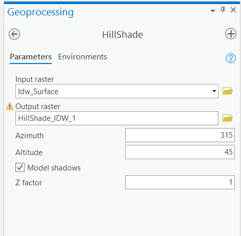
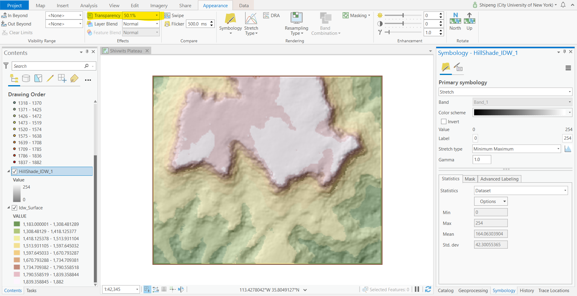
The Hillshade tool produces the following data.
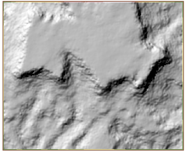
To get a better visual effect, we can increase the transparency of the hillshaded map and lay it on the top of the original surface data.
Try the same process with Spline and Kriging methods.
Questions: Can you visually identify the differences among those maps? By principles, do they have the exact same elevation ranges? Which method(s) can keep the original elevation values, and which method(s) cannot?
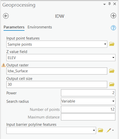
Exercise 2: Explore options in IDW
Each of the interpolation tool has many options. Using IDW, we explore how those options can possibly impact the results.
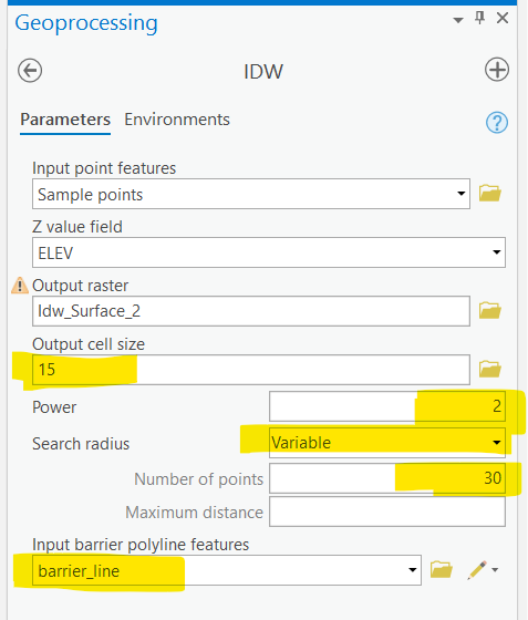
Vary the parameters of the cell size, power, search radius (number of points or maximum distance), and barrier.
Questions: From the experiment with different power settings and search radius, what kinds of settings give us smoother results, higher power or lower power, bigger radius or smaller radius, more points or less points? Do smoother surfaces from interpolation always mean better results? How do cell size and barrier polylines impact the interpolated surfaces? Use as many of your maps (colored and hill-shaded) as necessary to illustrate your answers.
Exercise 3 Create 3D Scene from the raster surface
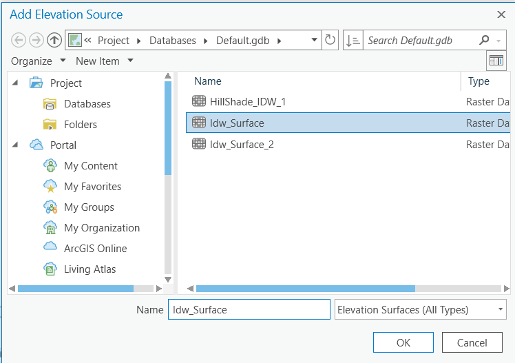
In task 2, we used TIN as elevation surfaces for 3D visualization. Here, we will use the raster elevation interpolated from points as surfaces in 3D visualization.
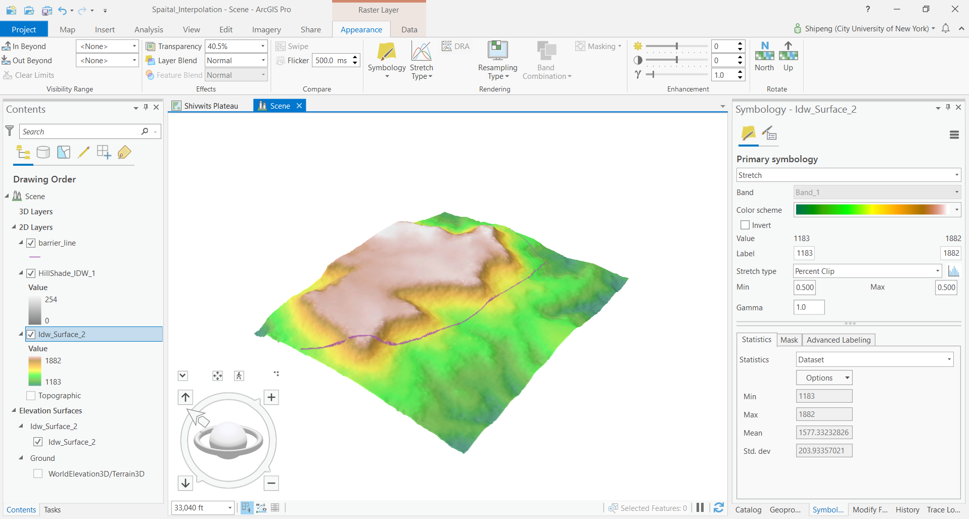
The process is almost identical to TIN except that we need to choose the raster elevation as the elevation source. Once the surface is set, others are the same as using TIN.
Questions: Create a visually appealing 3D map and export it to a high-resolution PNG image. How would you compare the colored, hill-shaded 2D map with the “3D” map? What are their differences in terms of application scenarios?
III. Instructions and Tips
The assignment must be typed and prepared in word-processing software, as hand-written work will not be accepted. The assignment answer file must be submitted through CUNY/Hunter Blackboard (bb.hunter.cuny.edu). Do NOT zip your document, do NOT send email to submit answers, and do NOT submit your data unless being asked to do so. If you have trouble using Blackboard, please contact the Hunter Help Desk.
The following file naming rule is used for this assignment when you submit the answers.
GTECH_732_361_L05_CUNY_ID.doc|docx|txt
L05 means lab 05. Do not omit the zero in the; otherwise, there would be file ordering problems on my end. Change the CUNY_ID (the [FirstName].[LastName][two digits]) to your owns.
Thank you!