Lab 03: Point Pattern and Cluster Analysis
GTECH 36100 GIS Analysis
GTECH 73200 Advanced GeoInformatics
Point Pattern, Clustering, and Spatial Autocorrelation
I. Objectives
For this week, we are learning descriptive point pattern measures, distance-based point pattern analysis, cluster analysis, and spatial autocorrelation. Spatial pattern analysis methods assess the relationships between values and locations of points or polygons using some form of distance or association measures. These measures are commonly compared with random spatial patterns to draw statistically robust conclusions. By measuring distances among points in a point set, we can determine if the points are more clustered or more dispersed than a random dataset. As such, we can statistically infer the spatial pattern of the point set.
Additionally, we can also use global and local spatial autocorrelation measures to identify clusters and hotspots (cold spots), which are very helpful in particular applications like crime analysis. When we need to address both values and locations, the spatial weight matrix is often required to represent the spatial relationships among points or polygons. In spatial statistical and regression analysis, GIS professionals would be very helpful if they can create spatial weight matrices based on various conceptualizations such as contiguity, indifference zone, and distance decay.
II. Lab Tasks and Requirements
For this week, you should also start planning your course project. To help on that, this lab will address some aspects of the course project planning, from data collection, to assembly, to visualization, and to analysis.
Task 1: Data Collection and Assembly
For this lab, we will analyze the spatial pattern of crimes in one of the boroughs in the New York City. As almost all GIS projects start with data, we must first collect data on crimes. For all the lab assignments so far, you are given relatively clean data. But here we will dive into the data collection, cleaning, and processing.
Step 1 Download Crime Statistical Data from NYC OpenData
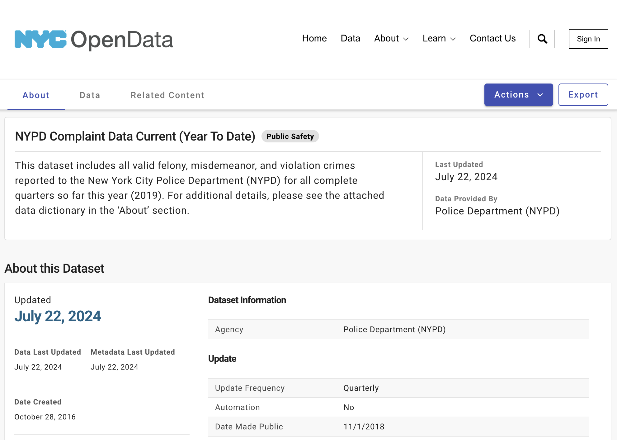
Visit NYC open data portal. Search “Crime Data” or “NYPD Complaint Data” and use the “NYPD Complaint Data Current YTD” entry. This dataset contains all the crimes reported by NYPD and most of the data records have Longitude and Latitude for mapping.
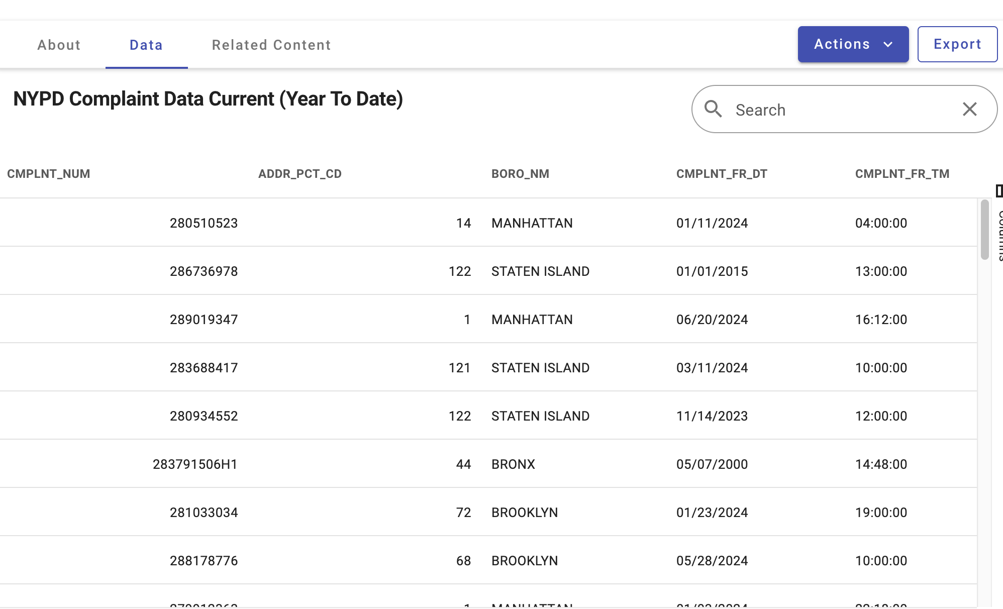
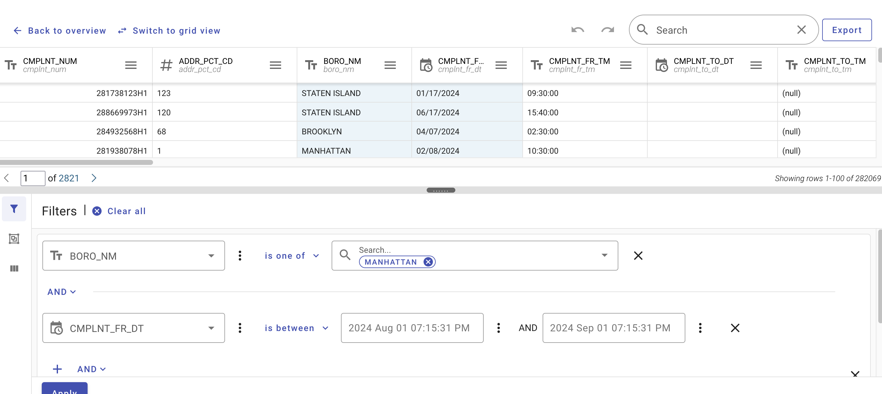
After clicking on “View Data”, we can open the data online for view. Although the website provides filters to select specific subsets of the data, we would rather to download all the data in CSV format and process the data in ArcGIS. Of course, if the dataset is too big, applying filters on the website would be recommended. Note that you can choose a (sub)dataset that you are interested in. No need to exactly replicate the steps in this document as it was done a few years ago.
This same dataset is also mapped on the portal as Crime Map and NYPD Complaint Map
From the mapping pages, we can also download the same dataset.
Step 2 Process the Downloaded Data
Now, we need to create a new file geodatabase and import the CSV into the geodatabase. Remember, most files that we download from the Internet are for exchange. They are not good for serious processing works. In the case of ArcGIS, always use a geodatabase.
Just create a new file geodatabase in Catalog and Import the CSV file into the geodatabase. The CSV file is a spreadsheet file. So, it is a table (only attributes), not a feature class. Also make this geodatabase as the default one. Note that we have learned these geodatabase-related steps before. If you don’t remember them, you can go back and check out the earlier lab tutorials.
After this, you should have one file geodatabase with the small home icon indicating it is the default one and a single table in the geodatabase. Take a screenshot of the geodatabase in the Catalog window.
Now let’s create a feature class (map layer) for a borough of NYC. I did Brooklyn, December 2017! You can choose a different borough and year, if you like.
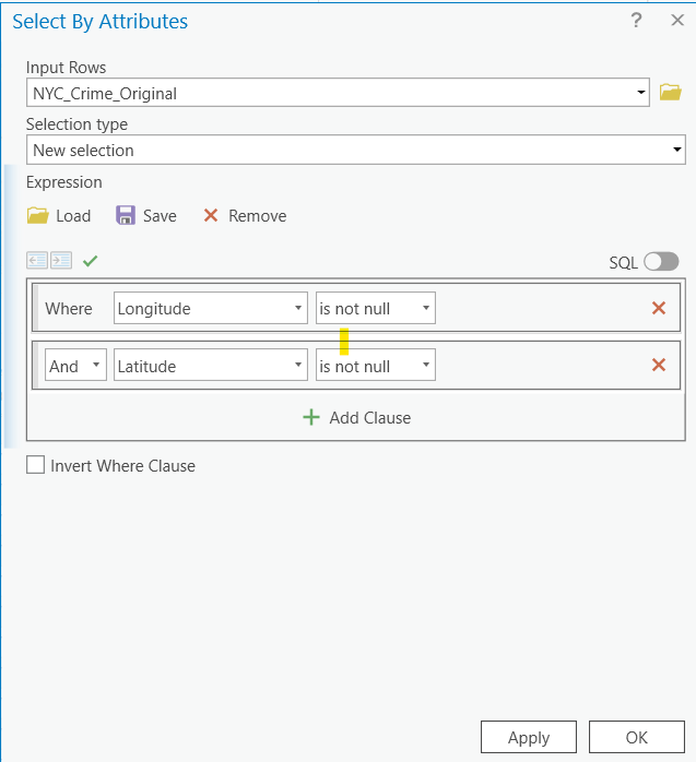
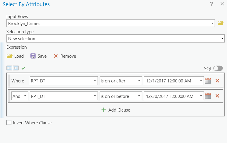
But first, we have to clean up the data a little bit and narrow down to this particular borough. Open the table that you just imported from the CSV file (assume its name is NYC_Crime_Original). Browse your data, so you have an idea how the data look like. Then open “Select by Attributes”.
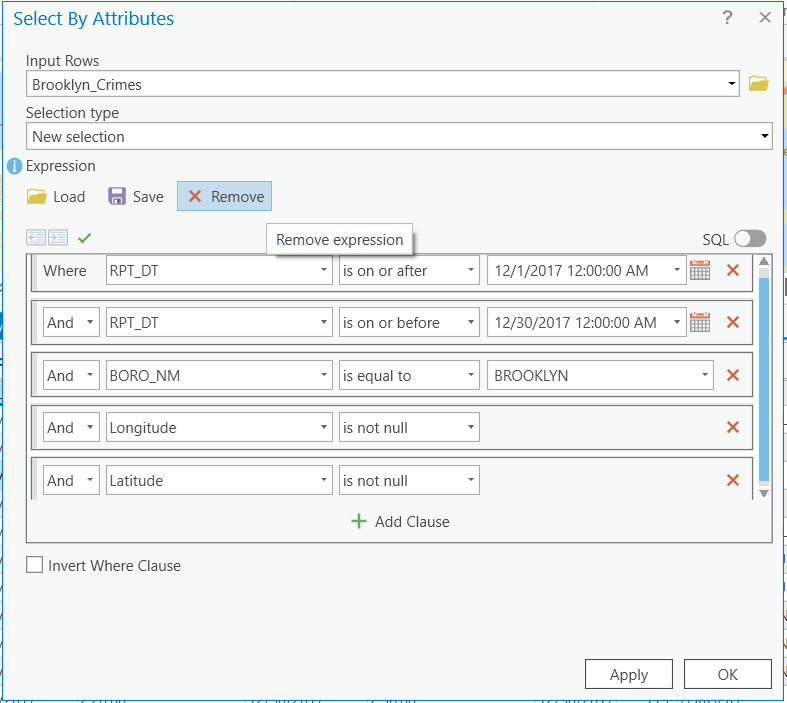
Now, we need to specify what we want to select. When you were browsing the data, you might have noticed that there were a lot of “Null” values in the X, Y Coordinates and Longitude and Latitude fields. For GIS works, we always want to have valid coordinates, so we must remove those data records without locational information. That is our first step: select those with valid coordinates. Using an expression like “Longitude IS NOT NULL AND Latitude IS NOT NULL”, we can select records with valid coordinates. Be patient as the dataset is very big! All the elements in the selection statement/expression can be chosen by clicking or double-clicking on certain items. In other words, we do NOT need to type anything using the keyboard for this.
After the selection, we can right click on the NYC_Crime_Original layer and export the “SELECTED FEATURES” into a new table in the default file geodatabase, say as NYC_Crime.
Now we can continue to select Brooklyn and December, 2017 from the NYC_Crime table. You can do this step by step: first, select Brooklyn using the BORO_Name field. Export the selected into a new table.
Then we can use the RPT_DT field to select specific dates from the newly exported table. Note that you don’t need to type in anything in the expression.
Export the selected records into a new table again.
Now, you have to select FELONY from the LAW_CAT_CD field as we do not want to examine MISDEMEANOR or VIOLATION type of crimes. I leave this step completely to you. Remember to export the selected records into a new table.
We can certainly combine all the selections in one single step; however, using multiple steps gives us many intermediate results. We also have the opportunity to check every step and to roll back only one small step if something is wrong. Of course, once you get more familiar with all the selection expressions/statements, you can absolutely do it in one single step to save time and the storage space.
Step 3 Mapping the data
Before we move to the next step, make sure your final table is for Brooklyn, in December 2017 or your own choice of borough/period combination, with valid coordinates, and only FELONY type. If the table contains anything otherwise, you have to check the steps above. It is worth to note that after every data processing or analysis step, we should verify the results and make sure they are good before we move to the next step. It would be disastrous that you find errors in the final or later steps but do not know which step caused the error. In that case, you probably have to redo all the steps, which is very costly.
Although we processed the data, they are just tables, not GIS layers in ArcGIS. So, we have to map the table data. In order to do that, we must have two coordinate fields (X, Y or Longitude, Latitude) of numeric types (integer, float, or double, not text or string). Note that the current Longitude and Latitude fields in the table are text/string, not numeric because there were non-numeric values in the original CSV when we imported the data into geodatabase.
We must convert these two fields to numeric, or double specifically. In ArcGIS, it is not possible to directly convert the field from one type to another. We have to add new fields and then given them values in the new type.
Add two double type fields: Lon and Lat (make sure no other fields use any of these names).
Right click on the field that you want to update, i.e., Lon or Lat. Open Field Calculator. Set Lon to Longitude. Again, there is no need to type anything. Just use mouse to finish the work.
Once we have two numeric (double) type fields for Longitude and Latitude, we can create a point feature class from it.
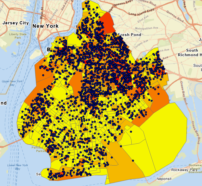
Recall the GPS exercise we did before and create a point layer from the Longitude/Latitude coordinates, which should look close to the figure below. Again, if you don’t remember the specific steps, please go back and check the previous lab tutorials again. Assuming NYPD collected the data using GPS technology, we still assign WGS 1984 coordinate system to the Longitude/Latitude.
Step 4 Add additional map layers and project the data to a local coordinate system
Find, download, and import the Kings County (Brooklyn Borough) Census tract boundary data to your file geodatabase and add the layer to the map document. Note this dataset was compiled from US Census data. This is one important skill that you also need to acquire. In the Geodatabase Lab, we have downloaded similar census boundary files from Census website. Revisit that part of the lab if needed.
You should have noticed that all our data are in geographic coordinate systems (decimal degrees) using WGS 1984. Although we can change the coordinate system in the ArcGIS Pro Map properties for visualization purposes, some Geoprocessing tools still require projected data to have more accurate measurements for distance, length, size, etc. For example, the Spatial Statistical tools like Mean Center in the next task recommend projected data as inputs. So, we must explicitly project our data into a local projection/coordinate system. As we learned in previous weeks, for New York City, the State Plane Long Island would be an appropriate choice.
Then we need to project the Brooklyn, 2017 December, Felony feature class into the same projection/coordinate systems. The tool is “Project”. Once we projected the data, we can import them into the feature dataset (Right click on the feature dataset, not the file geodatabase).
In the end, you should have at least two feature classes: felony crimes and census tracts in one NYC borough.
Task 2 Calculating centers, standard distance and ellipse
Step 1 Produce Mean Center for Felony Crimes
Now, search and open the Geoprocessing tool “Mean Center” or open it from Toolboxes \(\rightarrow\) Spatial Statistical Tools \(\rightarrow\) Measuring Geographic Distributions. This is a very simple tool that creates a point for the mean center of the input features.
Step 2 Calculate standard distance and ellipse
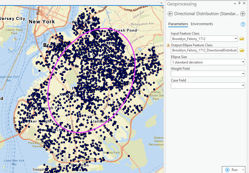
Although the mean centers of a set of features tell us the concentrated locations, they contain no information about the dispersion of the features. The standard distance measures how much the distances between the features and the center deviate from the average distance.
Using the “Standard Distance” tool, create circles(s) to represent such deviation. Similarly, run the “Directional Distribution” to calculate the standard deviational ellipse.
Task 3 Point Pattern Analysis
Step 1 Run the “Average Nearest Neighbor” tool and interpret the results.
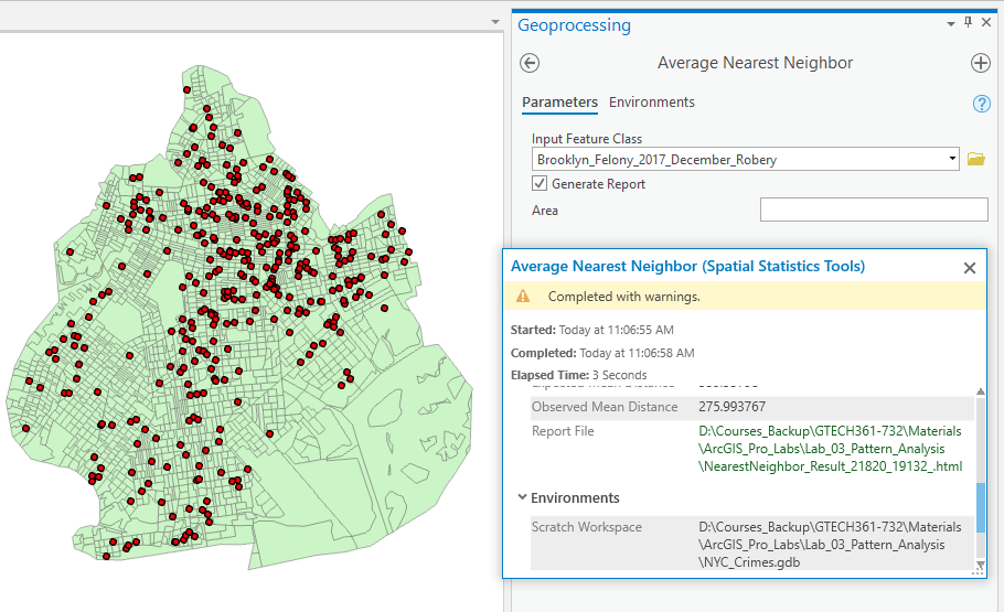
Note that the report link is in the results.
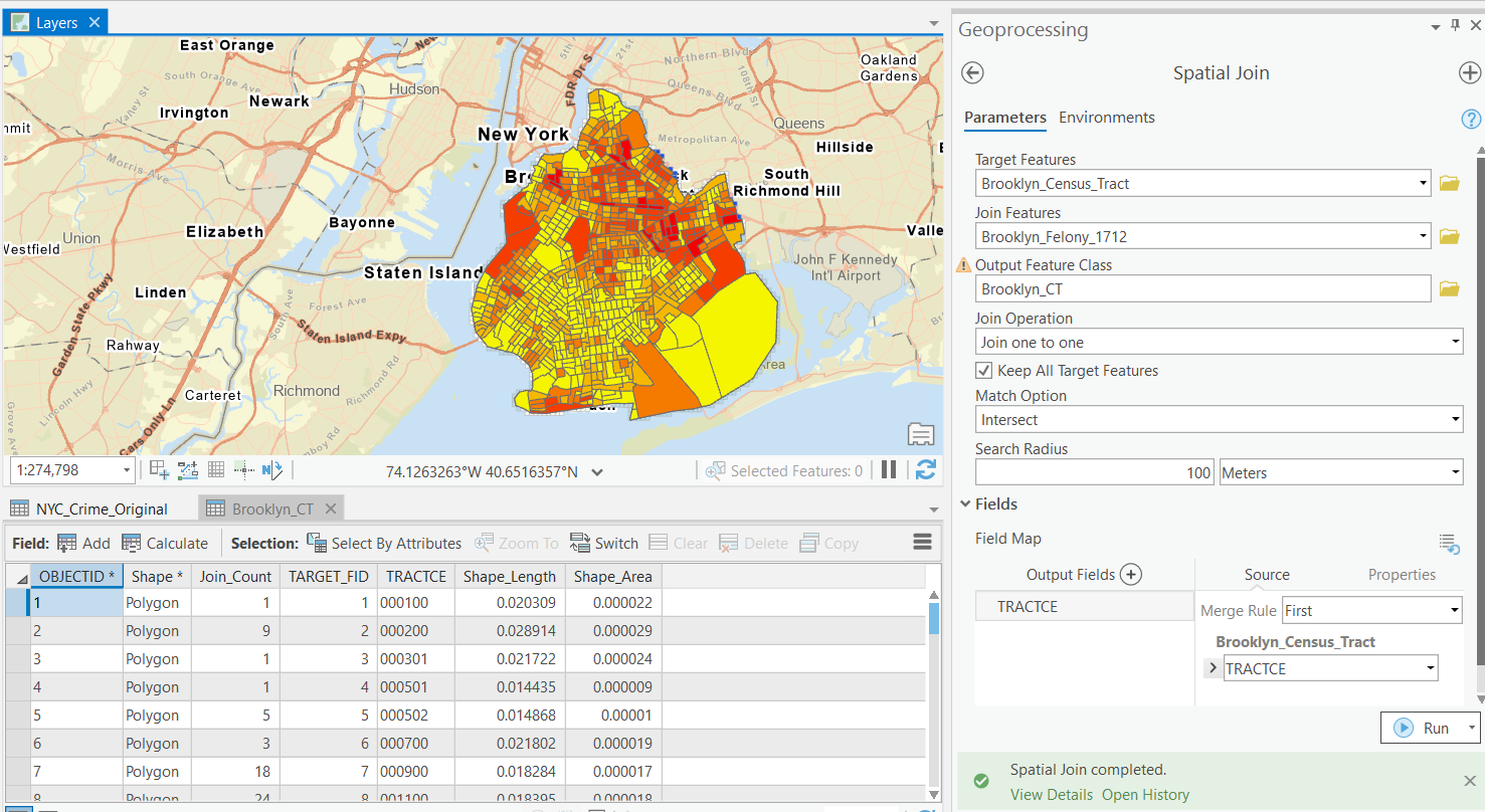
Step 2 Run a spatial join to get the number of crimes in each census tract.
Many pattern analyses are based on values in addition to locations. The spatial join will help produce those values for the following analyses.
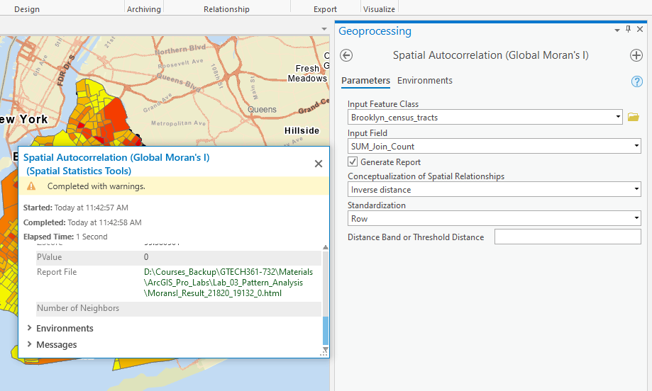
Step 3 Run Spatial Autocorrelation and interpret the results.
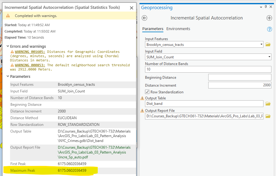
Step 4 Run Incremental Spatial Autocorrelation to find the optional distance band
One important conceptualization of spatial relationship is the distance band, where features within a certain distance are claimed near. However, it is very hard to know what distance to choose. The incremental spatial autocorrelation tool can calculate Moran’s I with a series of such distances, from which we can choose an optional distance that produces the highest spatial autocorrelation. In other words, this helps us find the maximum spatial autocorrelation.
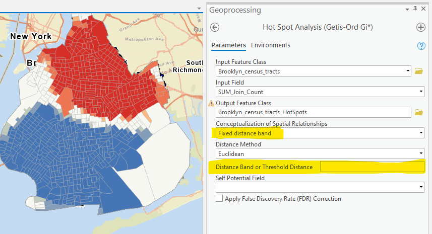
Step 5 Hot spot analysis
Run hot spot analysis using fixed distance band and inverse distance. For the fixed distance band, try two options. One is to use the default option, i.e., no inputs and let the tool choose one. The other is to use the one that produces the maximum spatial autocorrelation in Step 4.
Compare and interpret the results.
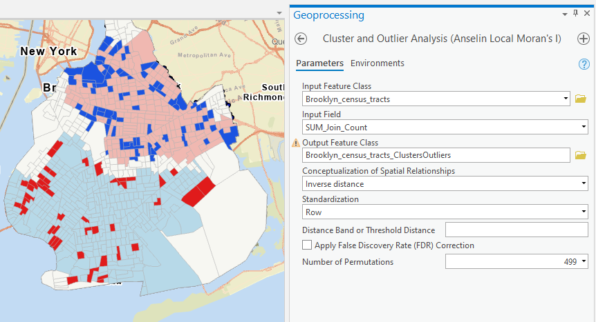
Step 6 Cluster and Outlier Analysis (LISA)
Run the tool and briefly interpret the results. How are they different from the results from hot spot analysis?
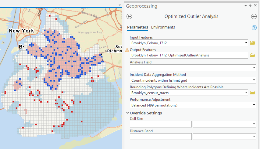
Step 7 Run Optimized Outlier Analysis
Interpret the results and compare them with cluster and outlier analysis (LISA or Local Moran’s I).
Make screenshots and copy the screenshots to a Word document. Submit one single document for the lab to the Blackboard. Please maximize your ArcGIS Pro Window when you make the screen shot (Press PrtScn/PrintScreen for the whole screen or Alt + PrtScn/PrintScreen for the active/focused window). Then paste the image into MS Word.
III. Instructions and Tips
The assignment must be typed and prepared in word-processing software, as hand-written work will not be accepted. The assignment answer file must be submitted through CUNY/Hunter Blackboard. Do NOT zip your document, do NOT send email to submit answers, and do NOT submit your data unless being asked to do so. If you have trouble using Blackboard, please contact the Hunter Help Desk.
The following file naming rule is used for this assignment when you submit the answers.
GTECH_732_361_L03_CUNY_ID.doc|docx|txt
L03 means Lab 03. Do not omit the zero in the; otherwise, there would be file ordering problems on my end. Change the CUNY_ID (the [FirstName].[LastName][two digits]) to your owns.
Thank you!