Lab 01: Geodatabases
Geodatabase Construction and GPS Data Processing
I. Objectives
During these two weeks, we learn the Geodatabases. We will create new File Geodatabases and populate them with data from various sources. Basically, a ESRI File Geodatabase stores various spatial data from GIS, RS (remote sensing), and GPS (Global Positioning System). To correctly perform spatial data integration, we must have a good understanding how the spatial data are measured and collected, particularly the geodetic datum, projections, and coordinate systems.
Note that in ArcGIS Pro, the projections and coordinates systems used by a Map could be different from the underlying spatial data layers. ArcGIS Pro automatically re-projects the underlying data to the projection of the Map on the fly for the purpose of correctly displaying the data. Yet, the underlying spatial data will not be changed or re-projected during this process.
With image registration and georeferencing (a fundamental topic in Remote Sensing courses), we can register satellite images and aerial photos on maps with correct locations. Increasingly, GPS, either dedicated GPS devices or embedded in smart phones, becomes the new data sources for GIS. GIS could use either separate points or routes/tracks from GPS receivers.
In this lab, we will learn to set projections, build Geodatabases, and integrate GPS data. We will also edit feature classes in file geodatabases and update the design and add validation rules to the database including subtypes, domains, and relationships.
II. Lab Tasks and Requirements
Download the lab assignment data. Unzip it to your working directory. Create a new ArcGIS Pro Map Project using the Map template.
Follow the instructions and complete the following tasks.
TASK 1 Build a Geodatabase
Create a new File Geodatabase in ArcGIS Pro Catalog Pane. In the Catalog window, select a folder, right click on it, and then choose New \(\rightarrow\) File Geodatabase. Do not use names like ‘aaa’, ‘bbb’, or ‘ksdj’. It is always good to make names readable and meaningful yet concise.
Right click on the new File Geodatabase. Choose the Import \(\rightarrow\) Feature Class(es). Import all the feature classes from the downloaded World_Reference geodatabase to the newly created file geodatabase.
Download the New York State Census Block Groups Boundary Shapefile from the Census website at Cartographic Boundaries or Census FTP Site for New York State
Unzip (extract) the zip file and import the feature classes/data layers into the new file Geodatabase.
| Extra Tips |
|---|
A Shapefile has multiple files (shp, shx, dbf, prj, xml, etc.). If you copy a Shapefile between computers, make sure you copy all of them, not just the single .shp file. There are three required files for a Shapefile: shp (the geometry/locations/coordinates), dbf (the attributes, it can be opened directly by Excel), shx (an index file for the geometry). If any of the three files is missing, ArcGIS would not be able to open the layer. The prj file, though not required, is also critical as it is the projection file. Without projection, ArcGIS would not know how to align the geometry with other layers, although it can still open the file and display it at the center of the computer screen. Another useful file is the xml file, which usually contains the metadata. |
Select the block groups within the five boroughs of the New York City using Select by Attribute. Make a new geodatabase feature class from the selection. Note this requires a new feature class in the file geodatabase. It is not enough to just make a new layer in the table of contents.
The county FIPS of the five NYC boroughs are 005, 047, 061, 081, 085.
Use screenshots, as many as necessary, to show your database (the Catalog View is a good tool to show geodatabase contents).
TASK 2 Set Map Projections.
Add the Circles, World30, and admin feature classes in the file geodatabase to your map. Change the ArcGIS Pro Map name to World Reference in Map Properties. Change the coordinate systems to Robinson, Eckert IV, Mercator, and Peters, which are arguably the four most popular projections for global mapping. When choosing projections, you are asked to use the ellipsoid-based geodetic datum, not the sphere-based one.
Also note that the Peters projection is copyrighted, and ArcGIS does not have the Peters in the list. The Peters projection is also known as Gall-Peters projection. It was intentionally created to make a direct contrast to the Mercator projection, which was popular in Western European classrooms and is still popular in the US today. Mercator increasingly enlarges countries farther away from the equator, which makes counties near the equator–mostly developing counties in Latin America, Africa, and South Asia–appear much smaller than their actual sizes. The Gall-Peters is an equal area projection, which means the size of an area on the map is proportional to its actual size. From Wikipedia, we can see the Gall-Peters projection is a cylindric equal-area projection with standard parallels at 45 degrees. From these parameters, we can create Gall-Peters in ArcGIS.
First, let us find the cylindrical equal area projection in ArcGIS Pro. You can search it or navigate to “Projected Coordinate Systems” \(\rightarrow\) “World”.
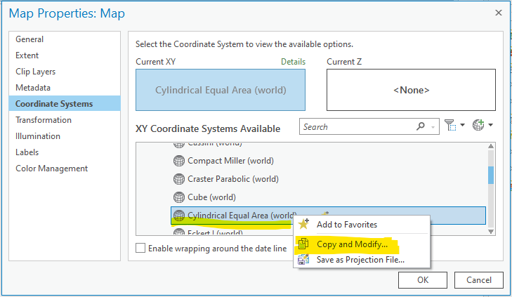
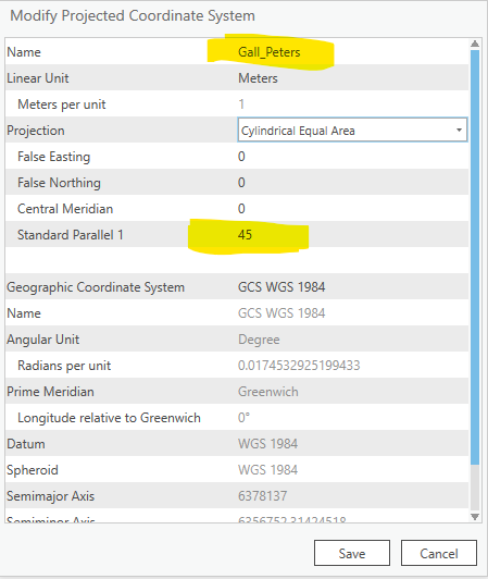
And we can see the default standard parallel for Cylindrical Equal Area is at 0 degree, i.e., the equator, not the 45 degree for Peters. Change it to 45 and name the new project as Gall_Peters. Now you have one of your own customized projected coordinate systems!
The most significant visual effect of the Peters projection is that Africa is much bigger than on a Mercator projection map. Today, most British schools adopt the Peters projection and the UNESCO also exclusively uses it for published maps. However, the Peters projection received a lot of critiques from cartographers due to its inferior aesthetics. Read a recent news report Why Map Historians are annoyed by the Boston Public Schools.
Zoom to the global extent and export a map for each of the four projections using menu Share –Map. Use PNG format and at least 300 dpi (the minimum dpi for quality print). Organize these four maps on a single Word page and explain in words about their differences in appearances, particularly distortions to sizes and shapes.
TASK 3 Import GPS/Coordinates data into Geodatabase
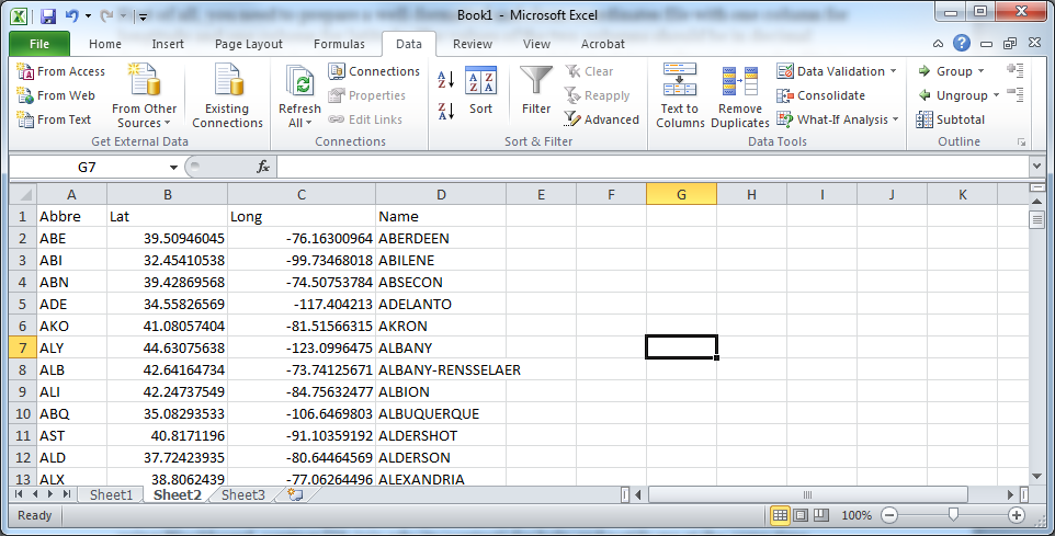
For this task, we will use the Armtrak Stations CSV file contained in the the downloaded data. Clean, convert, and process the data. Import them into ArcGIS Pro, and create a feature class for them. For extra practice, you can use the other examples of GPS data with separate points (Links or the data are in the “Sample Datasets” page of the lecture slides).
First of all, you need to prepare a well-formatted and clean coordinates file with one column for longitude and one column for latitude. The values of the two columns should be in decimal degrees. You can edit the file using Excel or other spreadsheet editing software. Save the file in CSV (comma separated values) or TXT format. ArcGIS can directly import Excel file if the system is set up properly, but CSV is a much simpler and safer option. It works all the time.
The file should have a header. Texts in the header should start with a letter, no space, no comma, no period, and no special characters. They would be the field names in the table. Empty lines should be removed. This often happens to the last line.
Second, import the CSV or TXT file into the file geodatabase as a table. Then you can create feature class from the table in the geodatabase using the XY Table to Point tool. Remember to set the coordinate systems for the input data. Again, GPS uses WGS 1984 Geographic coordinates.
Visually check if the data look correct. If anything looks not right, go back check the data and repeat these steps. It is very normal to go back and forth a few times to get things right.
Post screenshots to show their locations (export a map) and their projection/coordinate systems.
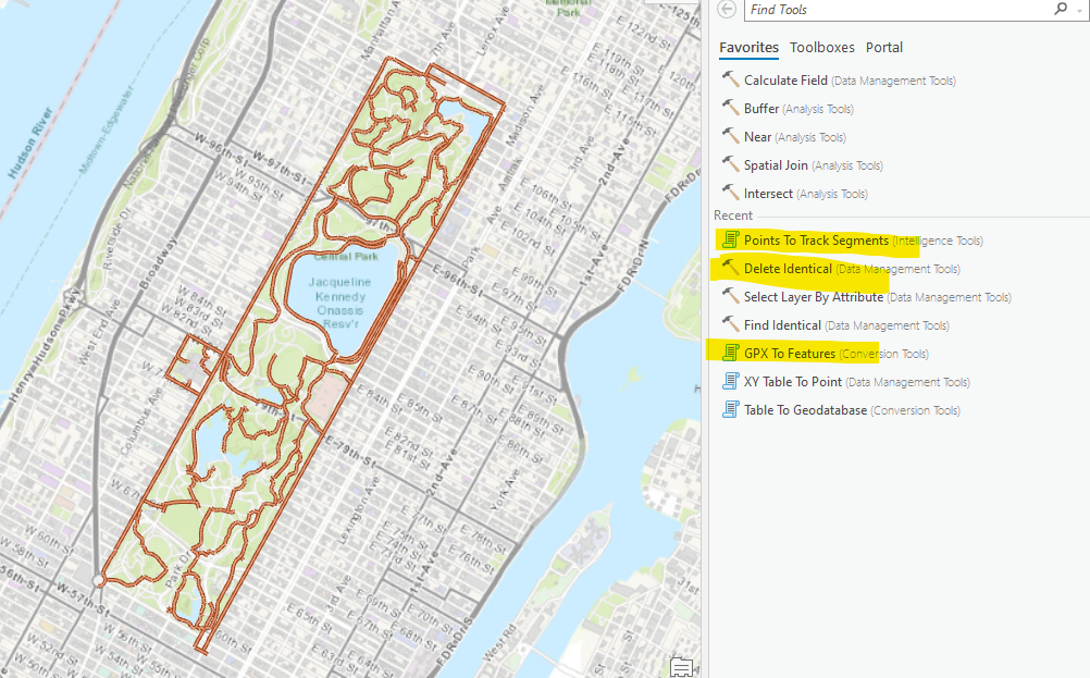
TASK 4 Import GPX File and Edit Data
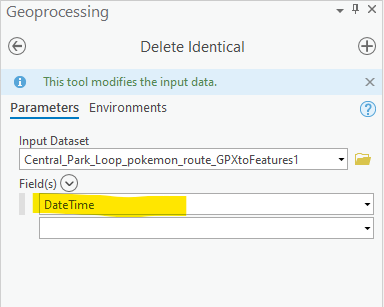
Use the “GPX to Feature” tool to import the central park GPX file as Points features. Use “Points to Track Segments” or “Points to Line” tool to create lines from the GPX points. These tools rely on a”Date” field to find the sequence of the points, assuming the person carrying the device moved along the trail in a consistent direction. However, the original GPX file has multiple points at the same time. As a result, the tools complain with errors as we demonstrated in the lab section. Apply the “Delete Identical” tool to remove those extra points at the same time and then run the “Points to Track Segments”.
As we discussed in the lab section, the purpose of the exercise is not really on those tools per se. Instead, it is to show a case of problem-solving. When we encounter errors running a tool, we should carefully read and make sense of the error message, search with the keywords in the error message, or ask for help with the screenshot of the errors.
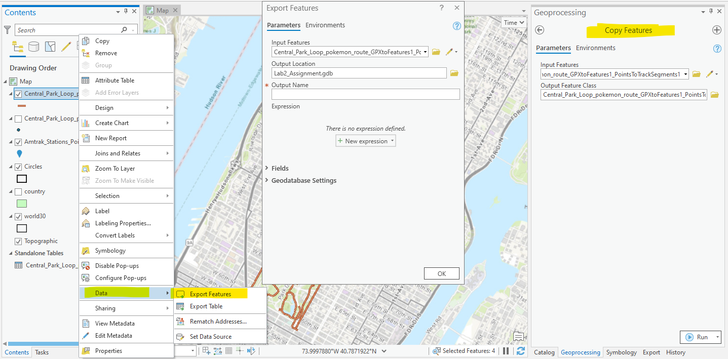
Save both feature classes in your file geodatabase using either the Export Features or the Copy Features tool.
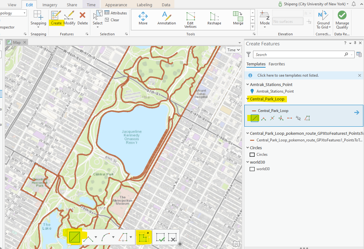
Using editing tools to digitize the Jacqueline Kennedy Onassis Reservoir in the Central Park. Create a new Feature class in the geodatabase for the central park (right click on the geodatabase in Catalog and then New Feature Class). You can use either line or polygon type for practice purposes, even though the polygon type is more appropriate for applications.
With the GPX tracks, the Trace tool in the editing is very efficient for a large part of the reservoir. For the general digitizing of lines, the Line and Freehand tool are more frequently used. For the general digitizing of polygons, the Polygon and Freehand are very useful. For the assignment, it is best to use all these tools.
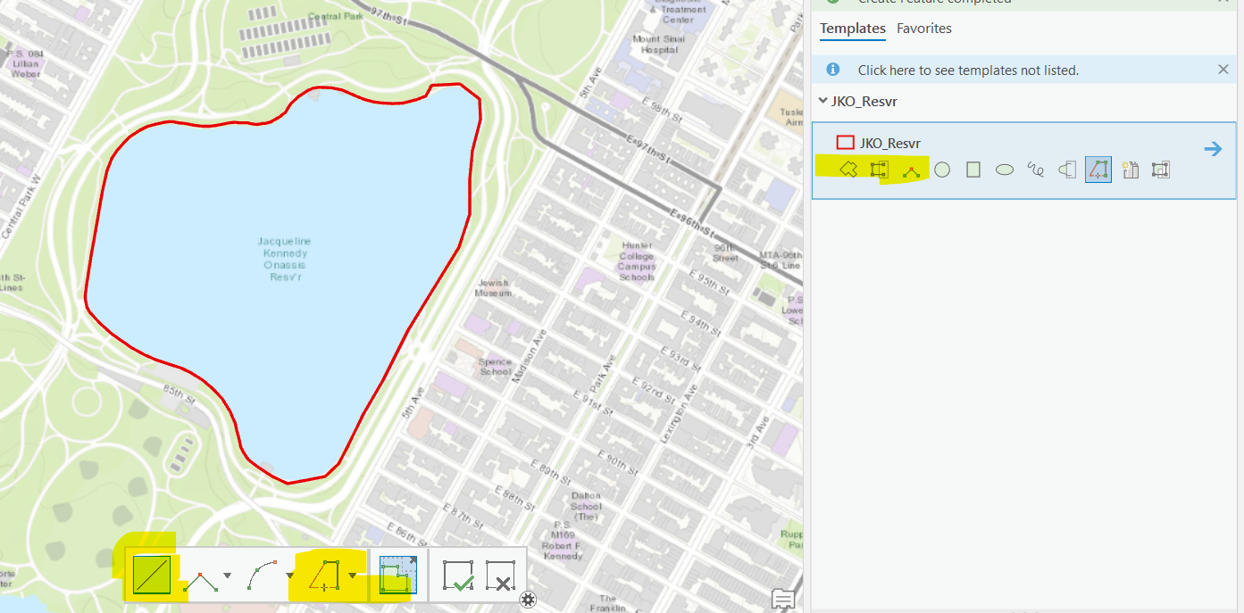
To editing an existing feature in the feature class, we must first select that feature and then select “Modify”. Once a feature is selected, we can edit its vertices and change its shape.
| Extra Tips |
|---|
| GPX, or GPS exchange format, is an XML file format for storing coordinate data. It can store waypoints, tracks, and routes in a way that is easy to process and convert to GIS data. Most hand-held GPS devices and smart phone GPS applications support GPX format exports. If you want to use GPS to collect data for GIS works, it is advised to export the data in GPX format. |
Use multiple screenshots to show your work, both the importing (show a screenshot of the file geodatabase in Catalog with the two layers of the GPS tracking points and lines) and the editing (show the edited GPS track inside the park).
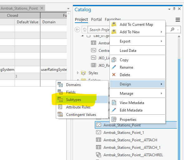
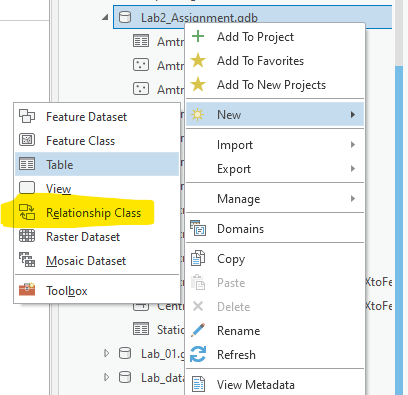
TASK 5 Domain, Subtypes, and Relationships
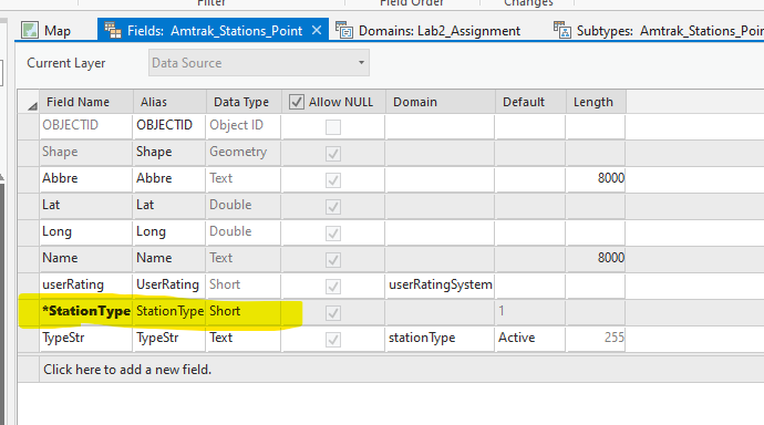
Essentially, we will create new fields in the Amtrak feature class. Apply domain, subtype, and relationships to them. For Amtrak stations, we will add subtypes and also allow storing user ratings and reviews. As one station could get zero to many reviews, they will have a one-to-many relationship.
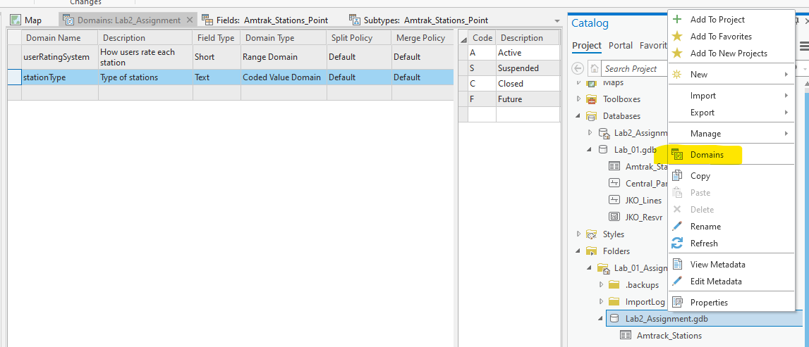
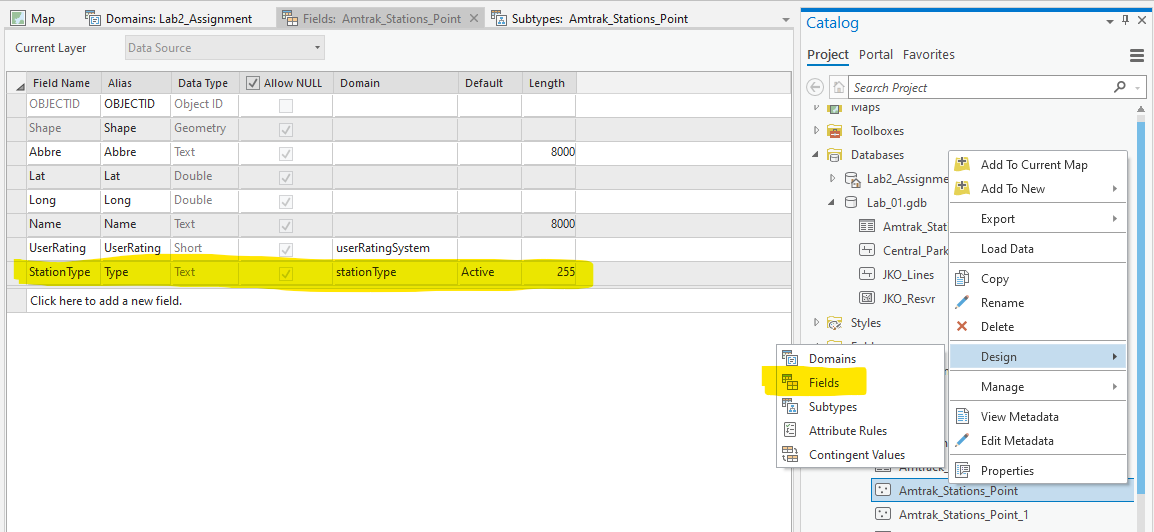
Station Type and Domains
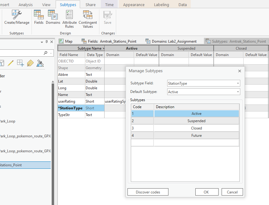
Add a StationType field of short integer. Create a subtype from this field with types of active, suspended, closed, and future (see Wikipedia on Amtrak stations). The default type is active.
User Ratings
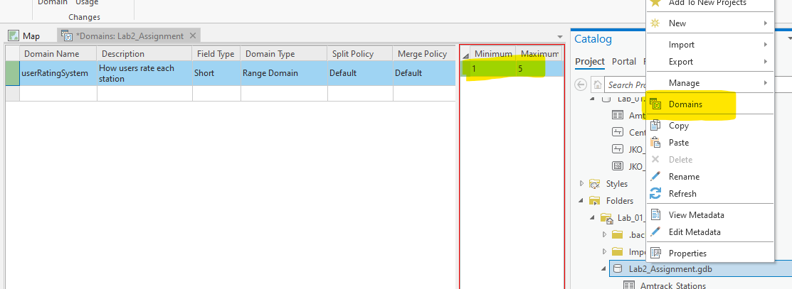
Create a UserRatingSystm domain of short type in the file geodatabase. Use a range domain from 1 to 5. Add a UserRating field of a short integer type and apply the domain. Null is allowed. No default values.
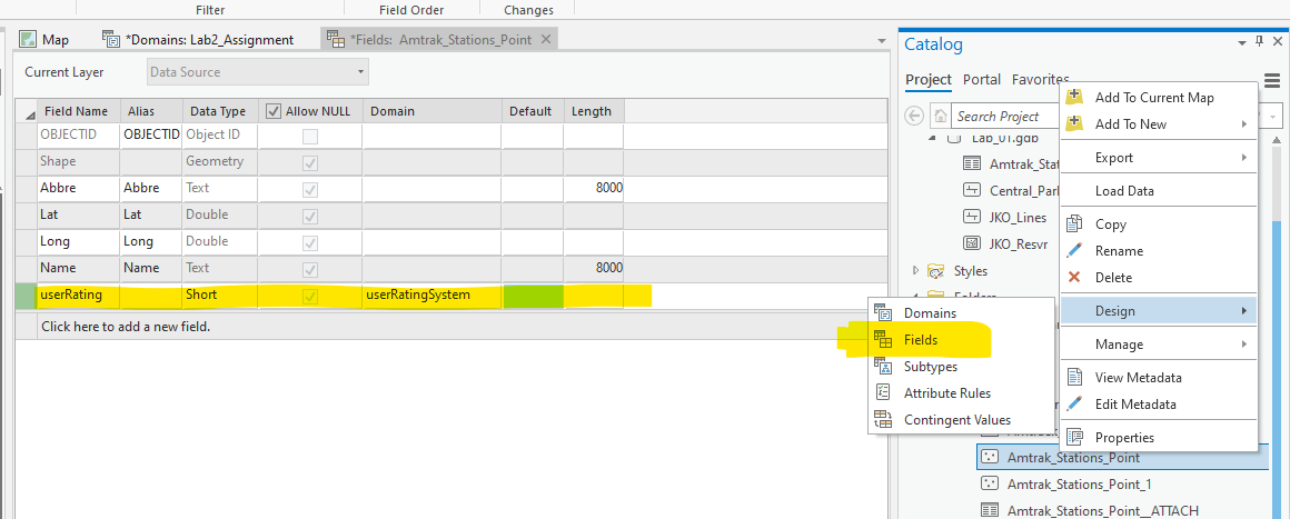
For the station type, we can also use coded value domain. Think about their differences from the subtype.
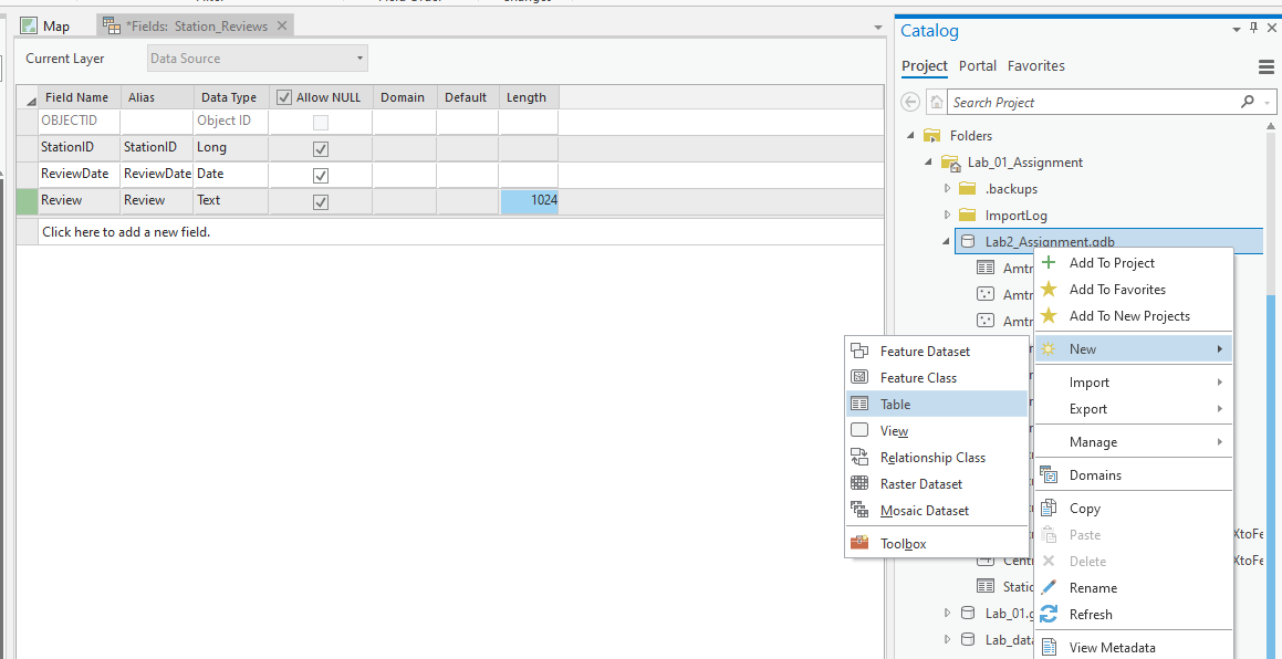
User Reviews
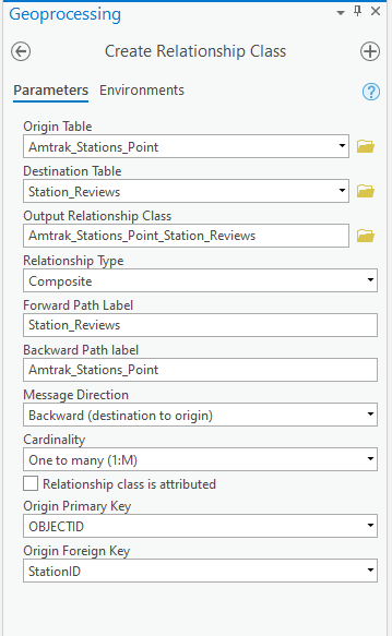
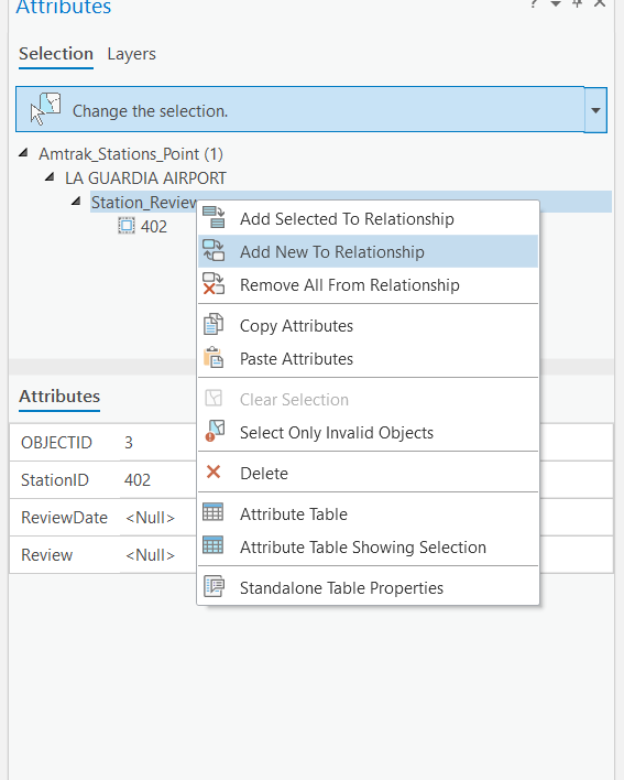
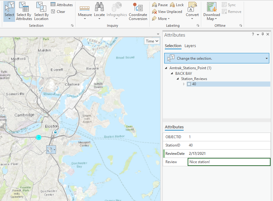
Add a review table with StationID, ReviewDate, and Review fields (see screenshot below). Create a one to many relationships between stations and these reviews. Basically, the relationship is that a review must be associated with a station and one station could have zero to multiple reviews.
With this relationship, we can add reviews when we edit the station attributes. Of course, in the real world, some computer code will add those reviews. But first, we must design the geodatabase to store those reviews appropriately.
Attachments
Allow attachment to the Amtrak station feature class. Search and download pictures for at least one station. Add those pictures as attachments.
TASK 6 Optimizing Geodatabases
Indexing is the de facto optimization standard for databases. It is a very powerful and effective tool that helps speed up the retrieval of records. Without indexing, a table is scanned sequentially and entirely to retrieve a particular record. So, if we have a dataset with n records, the worst-case scenario is that the record we are trying to locate is the last record in that table, and thus we need to search through n records in order to reach it. Imagine a feature class with a million features, and the time taken to visit each feature is 1 millisecond; this means we need 17 minutes to scan the entire dataset. Of course, the response time depends on the record you are looking for; if it is located at the beginning of the feature class, it will take less time to be located.
Indexing is pretty much similar to how you arrange your files alphabetically at your desk at work. To enable indexing, the geodatabase creates another structure for the attribute to be indexed. In this example, we will create an index for the Name column, which points all letters to their matching object IDs. Indexing works similarly with almost any field type, text, numbers, date, and even spatial data types. Indexes created on shape columns are called spatial indexes, which have the same concept as attribute indexes. Both of them shrink the query search domain to achieve greater performance.
To create an attribute index, perform the following steps:
Step 1: First, make a copy of your geodatabase in a different directory in case the current database is broken. Right-click on the Amtrak_Stations feature class, select Properties, and then select the Indexes tab.
The Attribute Indexes section shows the existing indexes on the feature class. As you can see, there is an FDO_OBJECTID index (the primary key), which is a very important index that cannot be removed. The geodatabase uses this index to uniquely identify each feature. When you click on FDO_OBJECTID, in the Fields section, you will see the field on which this index is created for.
Step 2: Click on Add… to add a new attribute index.
In the Add Attribute Index dialog, type in IND_NAME in the Name field. This is the index name. From the Fields available list, select the NAME field, which is the Venue’s Name column, and click on the right arrow icon to add it to the list.
The Unique and Ascending checkboxes are disabled by default for file geodatabases; however, they can be enabled for enterprise geodatabases depending on the underlying relational database system.
Step 3: Click on OK to close the dialog to return to the indexes form.
You will see that the IND_NAME index has been created on the NAME field, and now all queries against the NAME field will be optimized. Click on Apply and then click on OK to close the dialog and return to Catalog.
When you create a feature class, a spatial index is automatically created and optimized for that feature class. At any time, you can drop and recreate the spatial index by performing the following steps:
Step 4: Right-click on the Amtrak_Stations feature class and select Properties…
Click on the Indexes tab. In the Spatial Index section, click on Delete to delete the spatial index. Click on Create if you want to create the spatial index again.
Deleting and recreating the spatial reference is a good exercise on a geodatabase that is frequently edited, as that will ensure consistency in spatial querying.
Take a screenshot of the Indexes tab of the Feature Class Properties window of the Amtrak_Stations feature class.
At the geodatabase level, we can also compress or compact the GDB (Right click on a GDB in Catalog and in the Administration menu). Explain the differences between these two optimization approaches to the GDB. Refer to the following webpages for the details.
III. Instructions and Tips
The assignment must be typed and prepared in word-processing software, as hand-written work will not be accepted. The assignment answer file must be submitted through CUNY/Hunter Blackboard. Do NOT zip your document, do NOT send email to submit answers, and do NOT submit your data unless being asked to do so. If you have trouble using Blackboard, please contact the Hunter Help Desk.
The following file naming rule is used for this assignment when you submit the answers.
GTECH_732_361_L01_CUNY_ID.doc|docx|txt
L01 means Lab 01. Change the CUNY_ID (in the form of FirstName.LastName[two digits] such as John.Doe90) to your own ID.
Thank you!