Exploring the Geodatabase Data Model

The geodatabase is a data format introduced with ArcGIS® software. Since you're taking this course, you may be wondering, "What exactly is a geodatabase and why should I use one?"

This lab will introduce you to the basic features and functionality that a geodatabase provides. To really understand what a geodatabase is and how to put its powerful capabilites to work, however, you'll need to know about subtypes, domains, relationships, and more. Each of these advanced data model components can be implemented in a standard geodatabase.

If you don't understand the geodatabase terminology you just read, don't worry—you'll be introduced to these components in the labs that follow. For now, you'll start by getting familiar with the geodatabase itself.

Learning objectives

A student who completes this module will be able to:

• explain how the geodatabase stores geographic data
• understand the differences between the two types of geodatabases
• describe the three primary components of the geodatabase
• name other components that can be stored in a geodatabase
• create a raster dataset in a personal geodatabase
• access information about a geodatabase and its components

Test drive a geodatabase

Think of this first exercise as being like taking a new car out for a test drive. You'll try out a few features to see some of the functionality offered by the geodatabase. Using ArcMap, you'll work with attribute domains to make valid edits to features in a geodatabase. You'll also solve a problem affecting water mains in a geometric network.

If you have an ArcEditor or ArcInfo license, you can do two steps at the end of this exercise that show you how to use relationships and edit a network. If you're working with ArcView, just read through those steps and look at the View Result graphics to get an idea of the additional functionality supported by the geodatabase.

Estimated time to complete: 30 minutes

Step 1 Start ArcMap and open a map

Start ArcMap and choose to open an existing map.

Double-click Browse for maps and navigate to your Lab06 folder. Double-click CityWaterS.mxd to open that map document.

You see a map of a subdivision. This subdivision contains lots with homes on them, two wells, and water lines that are joined together to form a water network. The data for all of these layers is contained in a single geodatabase.

Step 1a: Start ArcMap and open a map

At the bottom of the Table of Contents, click the Source tab.

The path to the data source for the map layers displays at the top of the Table of Contents. You can now see that the source of the data shown in the map is a personal geodatabase named CityWaterS.mdb.

You may need to scroll or widen your Table of Contents to see the full path to the data source.

Step 1b: Start ArcMap and open a map.

Click the Display tab.

Step 2 Add a new well feature to the subdivision

A major advantage of storing data in a geodatabase is that you can validate edits made to the data.

If your Editor toolbar is not displayed, click the Editor Toolbar button to display it. If you like, dock the Editor toolbar to your ArcMap window.

From the Editor menu, choose Start Editing.

On the Editor toolbar, make sure the Task is set to Create New Feature. In the Target dropdown list, choose Wells. (If you're using ArcView, you will see only the Wells layer in the Target list).

Step 2a: Add a new well feature to the subdivision

Next, click the Sketch tool and click inside the southwest corner lot of the subdivision to add a well.

Step 2b: Add a new well feature to the subdivision

Step 3 Add attribute data for the new well

Now that you've created a new well feature, you need to add its depth attribute value.

On the Editor toolbar, click the Attributes button .

Tip: If your Editor toolbar is docked to the ArcMap window and you don't see the Attributes button, widen your ArcMap window.

In the Attributes dialog, the Depth value is currently shown as <null>.

Replace the null value with 50 (feet) for the well depth.

Step 3: Add attribute data for the new well

Close the Attributes dialog.

Step 4 Validate the attribute data

In the area where this subdivision is located, state regulations specify that residential wells must be between 40 and 120 feet deep. An attribute domain was created in the geodatabase to make sure that only lawful depth values are associated with residential well features.

In this step, you'll check to see that the well you just added, plus the two other wells, comply with state regulations.

Hold down your Shift key, then click the Edit tool and select all three wells. Make sure no other features are selected.

Tip: If you're having trouble selecting the wells without selecting other features, from the Selection menu, choose Set Selectable Layers. Make Wells the only selectable layer.

Step 4a: Validate the attribute data

From the Editor menu, choose Validate Features.

The well in the northwestern lot is selected and a message tells you its Depth value is not within the acceptable range.

Step 4b: Validate the attribute data.

Because this well's depth is actually 60 feet, you know there has been a data entry error. You'll edit the depth attribute for this well.

Click OK to close the message.

Step 5 Edit data and validate again

Open the Attributes dialog. Change the depth value for the selected well to 60.

Step 5a: Edit data and validate again

Close the Attributes dialog.

From the Editor menu, choose Validate Features again to make sure your edit is within the allowable range.

All the wells should now have valid values.

Step 5b: Edit data and validate again

Click OK to close the validation message.

Step 6 Display the Utility Network Analyst toolbar

Your next task is to solve a network problem using a geometric network that has been created in the geodatabase. The first five layers shown in the Table of Contents participate in the network.

Step 6a: Display the Utility Network Analyst toolbar

To access the network functions, you need to display the Utility Network Analyst toolbar.

From the View menu, choose Toolbars, then click Utility Network Analyst.

Step 6b: Display the Utility Network Analyst toolbar.

If desired, dock the toolbar to your ArcMap window.

Step 7 Add a junction flag

In this and the remaining steps, you will perform some basic network analysis. Don't worry about memorizing the process you follow here—remember, you're just on a test drive to see what the geodatabase can do.

First, you'll perform an upstream trace from the end of a water main back to the water tank, the origin of flow for this network. Before you can perform a trace, you need to add a junction flag at the water main location.

On the Utility Network Analyst toolbar, click the Add Junction Flag tool .

Your mouse pointer changes to a flag.

Using the graphic below for reference, click the Cap junction at the end of the 6-inch water main line to add a junction flag.

Step 8 Perform a trace operation

On the Utility Network Analyst toolbar, in the Trace Task dropdown list, choose Trace Upstream.

Click the Solve button .

The flow path from the water tank (the network source) in the northwest corner of the map to the junction flag you added displays in red.

Step 8: Perform a trace operation.

From the Analysis menu, choose Clear Results. Again from the Analysis menu, choose Clear Flags.

Step 9 Test network connectivity

Several water customers have called in to complain that their water pressure has suddenly dropped. You suspect a broken pipe, and you want to identify the pipe that is common to all the call locations.

Using the method described in the previous step, set three junction flags at the water meter locations shown below:

In the Trace Task dropdown list, choose Find Common Ancestors.

Click the Solve button .

The break is probably on the first highlighted pipe that is upstream from all the complaint locations.

Step 9: Test network connectivity.

From the Analysis menu, choose Clear Results. Again from the Analysis menu, choose Clear Flags.

If you are using ArcView to do this exercise, you will not be able to do the next two steps. Read through them, if you like, or skip to step 12.

Step 10 Remove lots and related houses (ArcEditor, ArcInfo users only)

The city is building a new reservoir and needs the land currently occupied by some of the lots in the southeastern portion of the subdivision. These lots and the houses on them will be removed from the subdivision to make way for the reservoir (but don't worry, the fictional homeowners are being well compensated for their forced relocation).

If you set the Wells layer to be the only selectable layer in step 4, change your selection settings so that both the Lots and Fittings layers are selectable.

On the Editor toolbar, click the Edit tool and hold down your Shift key. Select the eight lots as shown below.

Make sure no other features are selected.

Click the Delete button .

Step 10: Remove lots and related houses (ArcEditor, ArcInfo users only)

Notice that both the lots and the homes sitting on them have been removed from the subdivision. A relationship class was set up in the geodatabase between homes and lots. When the lots were deleted, the related homes were deleted as well.

Step 11 Edit the network (ArcEditor, ArcInfo users only)

Your final task is to edit the water main. Because the eight lots were removed, the length of the water main that served those homes needs to be adjusted.

The geodatabase maintains connectivity between features in a network. When you move a network feature, the features connected to it will also move.

Using the Edit tool, select the Cap feature at the end of the water main.

Drag the Cap to the left, to the end of the last lot, then click away from the feature to unselect it.

Step 11: Edit the network (ArcEditor, ArcInfo users only).

Step 12 Save your work

From the Editor menu, choose Stop Editing. Click Yes to save your changes.

Save the map document, then close ArcMap.

Conclusion

In this exercise, you were introduced to three geodatabase features: attribute domains, geometric networks, and relationship classes. Together, these features provide powerful tools for ensuring database integrity and finding answers to common GIS problems.

Explore the structure of a geodatabase

In this exercise, you'll get a different perspective on the geodatabase you worked with in the first exercise. This time you'll look at it in ArcCatalog.

ArcCatalog is the ArcGIS application used to create and manage geodatabases. ArcCatalog is also the place to go when you need information about the structure of a geodatabase: its feature datasets, feature classes, nonspatial tables, and the other components that it may contain.

This exercise will teach you how to access information about the structure of geodatabase components.

Estimated time to complete: 30 minutes

Step 1 Open ArcCatalog and create a connection to the exercise data

Open ArcCatalog.

You'll first create a connection to the exercise data folder for this course—by doing so, you'll be able to quickly get to the data for each module.

Click the Connect to Folder button and navigate to your Lab06 folder. Click the Geodatabases folder.

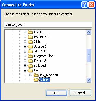
Step 1: Open ArcCatalog and create a connection to the exercise data.

Click OK to create the folder connection.

The new folder connection displays in the Catalog tree.

Step 2 Examine the geodatabase in the Catalog tree

In the Catalog tree, expand the folder connection you just created, then expand the Explore folder.

You see the personal geodatabase named CityWaterS.mdb that you worked with in the previous exercise.

Expand the CityWaterS.mdb geodatabase.

Step 2: Examine the geodatabase in the Catalog tree.

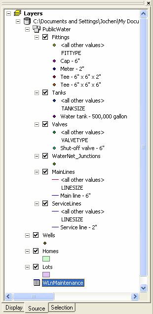
This geodatabase contains one feature dataset named PublicWater, three standalone feature classes (Homes, Lots, and Wells), one table of nonspatial data named WLnMaintenance, and a relationship class named HomesLots.

The relationship class establishes how the Homes features are related to the Lots features. You saw an effect of this relationship in the previous exercise when you deleted the lots and the homes were deleted automatically. You'll learn about relationship classes in Module 4 of this course.

Step 3 Examine the feature dataset

The PublicWater feature dataset contains the network features you worked with in the previous exercise.

Expand PublicWater to see its contents.

Step 3: Examine the feature dataset.

The first five items listed in PublicWater are user-defined feature classes. The last two items, WaterNet and WaterNet_Junctions, were created by the software when the geometric network was created.

All the components in the PublicWater feature dataset work together to form an integrated network that allowed you to trace the flow of water through the water lines and locate a broken pipe.

Step 4 Preview the Wells feature class

In the previous exercise, you created a new well feature and added attribute data for it. This data was stored in the Wells feature class. In this step, you'll find out more about this feature class.

In the Catalog tree, click the Wells feature class, then click the Preview tab on the right to preview the geography of Wells.

You see three well features. Each feature is stored as a row in the feature class table.

Note: If you didn't complete the first exercise, you will see only two wells.

Step 4a: Preview the Wells feature class.

In the Preview dropdown list at the bottom of the Preview area, choose Table.

The OBJECTID and SHAPE fields were automatically generated by the software. The Depth field is a user-defined attribute field.

Step 4b: Preview the Wells feature class.

Step 5 Examine feature class properties

In ArcMap, you can see features and their attributes. In ArcCatalog, however, you can get more information about feature classes.

Right-click Wells and choose Properties.

The Feature Class Properties dialog displays. Click the Fields tab.

The three fields in the Wells feature class table are listed along with the type of data each field can contain.

Click the gray box to the left of Depth.

The properties of the Depth field display in the middle of the dialog.

Step 5a: Examine feature class properties.

Notice that there is a domain called WellDepth associated with this field. You'll find out more about this domain in the next step.

Click the Subtypes tab.

If the well features had been grouped into subtypes, the subtypes would be described in this panel. However, you can see that the Wells feature class has no subtypes.

Step 5b: Examine feature class properties.

Click the Relationships tab.

1 Does the Wells feature class participate in any relationships?

Click Cancel to close the Feature Class Properties dialog.

Step 6 Examine the geodatabase properties

What properties are associated with the geodatabase as a whole?

To find out, right-click CityWaterS.mdb and choose Properties.

Click the Domains tab.

You see information on the domains associated with the geodatabase.

Step 6: Examine the geodatabase properties.

At the top of the dialog, three domains are listed. The first two domains, AncillaryRoleDomain and EnabledDomain, are part of the geometric network. The third domain, WellDepth, is the domain you used in the previous exercise to validate well depths.

Click the gray box to the left of WellDepth.

The domain properties display in the middle of the dialog.

2 What is the minimum value for a well's depth, as specified by this domain?

You'll learn how to create attribute domains in Lab 9.

Close the Database Properties dialog.

Step 7 Create a standalone feature class

There are several ways to create a feature class in a geodatabase. In the next two modules, you'll get lots of practice creating feature classes. For now, you'll try one method.

Right-click CityWaterS.mdb, click New, then click Feature Class.

The New Feature Class dialog displays.

For Name, type Roads.

Step 7a: Create a standalone feature class.

Click Next.

Accept the default keyword configuration option and click Next.

In the third panel, click the gray box next to SHAPE.

In the field properties area, notice that the default Geometry Type is polygon.

Click in the column next to Geometry Type and choose Line in the dropdown list.

Step 7b: Create a standalone feature class.

Next, you'll add an attribute field.

At the top of the dialog, click in the empty cell below SHAPE. Type RoadName and press Tab to move to the Data Type column.

The default data type is Text, the appropriate data type for this field.

Step 7c: Create a standalone feature class.

Click Finish.

The new Roads feature class is created and displays in the Catalog tree.

Step 7d: Create a standalone feature class.

Preview the table for the Roads feature class.

Step 7e: Create a standalone feature class.

Notice the SHAPE_Length field. The geodatabase automatically stores and maintains length values for line features.

The feature class structure has now been created. The next step would be to add its features and attribute data using the ArcMap editing tools. You'll learn how to create features and attributes in Module 3 of this course.

Step 8 Explore on your own

In steps 4 and 5, you learned how to use Preview and the Properties dialog to find out more about the Wells feature class. Use the same methods to get information about the other CityWaterS geodatabase components you see listed in the Catalog tree.

Here are a few suggestions to get you started:

• Look at the properties for the WLnMaintenance table. How do nonspatial table properties differ from those for a feature class?
• Expand the PublicWater feature dataset and examine the properties of its feature classes. In particular, examine how the feature class subtypes are defined.
• Not all the items you see in the Catalog tree can be previewed. Which items can't be previewed and why do think this might be?

Don't worry if you can't find the answers to these questions now. You'll learn them in the modules that follow.

When you're finished exploring the geodatabase, close ArcCatalog.

Conclusion

As you discovered in this exercise, you can get a lot of information about a geodatabase, its structure, what its various components look like, and how they work together by using ArcCatalog's Preview tab and Properties dialogs.

Throughout this course, you will work with both ArcCatalog and ArcMap to create and edit geodatabase features.

Explore raster data

In this exercise, you will get a brief introduction to working with rasters in a geodatabase.

Using ArcCatalog, first you will create a new raster dataset in a personal geodatabase and examine a raster catalog that has already been created. Then, using Windows Explorer, you'll look at the differences between the file structure for a managed raster and an unmanaged raster.

Estimated time to complete: 20 minutes

Step 1 Open ArcCatalog and navigate to the exercise data

Start ArcCatalog and expand your Geodatabases folder connection. Expand the Explore folder.

You see the AlachuaCounty.mdb personal geodatabase.

Expand AlachuaCounty.mdb.

Step 1: Open ArcCatalog and navigate to the exercise data

This geodatabase contains one feature dataset (Administrative), a raster catalog (StudyArea2) which you'll explore in later steps, and a standalone feature class (MajorRoads).

Step 2 Examine raster properties

In the next step, you will create a raster dataset in the AlachuaCounty geodatabase. The data stored in this raster dataset will be a mosaic of the three MrSid images: aerial_east.sid, aerial_south.sid, and aerial_west.sid.

Before creating the raster dataset, you'll take a look at the images.

In the Catalog tree, click aerial_east.sid, then click the Preview tab to see the image.

Step 2a: Examine raster properties

In the Catalog tree, right-click aerial_east.sid and choose Properties.

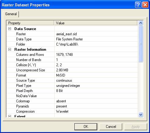
Step 2b: Examine raster properties.

Scroll down through the dialog and examine all the properties for aerial_east.

3 In what coordinate system is this image stored? Hint: Look next to Spatial Reference.

Close the dialog.

To mosaic images together into a single raster dataset, each of the images must have the same properties (number of bands, cell size, format, and spatial reference).

Preview the aerial_south.sid and aerial_west.sid images and examine their properties.

4 Do these images have the same properties as aerial_east?

Another criteria for mosaicking is that the images must be adjacent. If you were to add these three images to ArcMap, you would see that they overlap, as shown in the graphic below.

The overlaps will be removed when you add the data to the raster dataset.

Step 3 Create a new raster dataset

There are several ways to get raster data into a geodatabase. The method you will use in this step and the next is to create an empty raster dataset and then load the three images into it.

In the Catalog tree, right-click AlachuaCounty.mdb, choose New, then click Raster Dataset.

The Create Raster Dataset tool opens. If you like, you can resize the tool dialog.

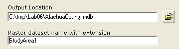
In the box under "Raster dataset name with extension," enter StudyArea1.

Step 3a: Create a new raster dataset.

The defaults for cellsize, pixel type, and number of bands are appropriate, so you do not need to change them. The coordinate system information will be provided by the images you add to the raster dataset.

Click OK.

The progress window shows the status of the processing. When the process is complete, close the progress window.

The new raster dataset has been added to the geodatabase.

Step 3b: Create a new raster dataset.

Step 4 Load the raster images

In this step, you will load the data from the three images into the StudyArea1 raster dataset.

Right-click StudyArea1, choose Load, then click Load Data.

The Mosaic tool opens.

You need to specify the three images that you want to load. The easiest way is to drag and drop the images into the tool from the Catalog tree.

Move your Mosaic tool dialog so that you can see both it and your ArcCatalog window.

In the Catalog tree, click aerial_east.sid and drag it into the Input Rasters box in the Mosaic tool.

Drag aerial_south.sid and aerial_west.sid into the box.

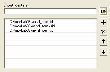
Step 4: Load the raster images.

You will accept all the default options for mosaicking the image data.

Click OK.

When processing is complete, close the progress window.

The image data has been added to the raster dataset.

Step 5 Preview the new raster dataset

In the Catalog tree, click StudyArea1 and preview the new image.

Step 5a: Preview the new raster dataset.

A new, seamless image has been created from the three image files. Notice the oval area in the center of the image—this is a wetlands area. Notice also that the areas of overlap among the three images have been eliminated in the new image.

Right-click StudyArea1 and choose Properties.

Step 5b: Preview the new raster dataset.

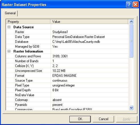
Under Data Source, you can see that the raster dataset is being managed by the geodatabase.

Notice under Raster Information that the format is ERDAS IMAGINE.

Remember that a personal geodatabase references raster data. When you load data into a raster dataset in a personal geodatabase, ArcCatalog mosaicks the data, saves the mosaic as an ERDAS IMAGINE file (.img), and stores the file in a folder that has the same name as the geodatabase. You don't see this folder in ArcCatalog.

In step 9, you'll use Windows Explorer to examine the file structure of the data referenced by the StudyArea1 raster dataset.

Close the dialog.

Step 6 Examine raster catalog properties

You'll now explore the second way that the geodatabase references raster data—a raster catalog.

A raster catalog named StudyArea2 has already been created in the AlachuaCounty geodatabase.

In the Catalog tree, click StudyArea2 and preview the raster data.

Step 6a: Examine raster catalog properties.

All the images in the catalog are displayed. Notice that unlike a raster dataset, the images loaded into a raster catalog don't have to be adjacent.

Preview the table for StudyArea2.

Step 6b: Examine raster catalog properties.

A raster catalog is a collection of rasters. Each record in the table corresponds to one raster. The Raster column stores the reference to the image files. The Shape_Length and Shape_Area fields are added by the geodatabase to store the perimeter and area of the raster footprints.

The StudyArea2 catalog contains six rasters.

Click the Contents tab.

Step 6c: Examine raster catalog properties.

The names of the referenced rasters are also listed here.

On the right side of the Contents tab is the Expand/Contract Window button.

Click the button to expand the window.

Step 6d: Examine raster catalog properties.

The footprints for all the rasters in the raster catalog are shown in the Overview tab.

Step 7 View raster properties in the catalog

Using the Contents tab, you can access information about each raster in the raster catalog.

In the Contents tab, under Name click doqq.jpg to select the image.

Step 7a: View raster properties in the catalog.

The Overview tab shows the selected image.

Click the Selection tab to see a larger view of the selected image.

Step 7b: View raster properties in the catalog.

You can also access metadata, properties, and a list of bands for each raster in the catalog.

In the dropdown list at the bottom right corner, choose Properties.

Step 7c: View raster properties in the catalog.

You see the properties for the selected raster.

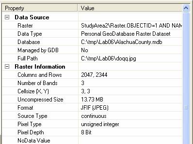
Under Data Source, notice that this raster is not managed by the geodatabase (its "Managed by GDB" property is No). Because the data is not managed by the geodatabase, if you were to copy the geodabase to a different location, the referenced images would not follow.

Notice also under Data Information that the format is JPEG, not ERDAS IMAGINE. When it is not managed by the geodatabase, raster source data remains in its original format instead of being converted to .img format.

Under Raster Information, notice that this image has three bands and the cell size is 3,3 (each pixel in the image represents 3 x 3 meters on the ground). You'll compare this information to another image in the next step.

Step 8 Examine another raster in the catalog

In the Contents tab under Name, click aerial_2.sid to view its properties. You may need to widen the Name column to see the full raster filenames.

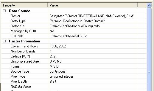
Step 8a: Examine another raster in the catalog.

Notice that this image has only one band and the cell size is 2,2.

Unlike rasters added to a raster dataset, rasters in a raster catalog can have different properties. To be viewable, though, all the rasters in a raster catalog must have the same spatial reference.

From the dropdown list, choose Geography. Click the Overview tab.

Step 8b: Examine another raster in the catalog.

This image overlaps the image you examined in the previous step. In a raster dataset, areas of overlap are eliminated. In a raster catalog, the data for all the rasters is preserved.

To preview both images, hold down the Ctrl key and click doqq.jpg.

Step 8c: Examine another raster in the catalog.

Step 9 Compare managed and unmanaged rasters

In this exercise, you have worked with both managed (StudyArea1) and unmanaged (StudyArea2) raster data.

To understand the differences in how the data is stored, you'll look at the data in Windows Explorer.

Minimize ArcCatalog.

Open Windows Explorer and navigate to your Lab06 folder. Expand the Explore folder.

Step 9a: Compare managed and unmanaged rasters.

You see a folder with the same name (but with an .idb extension), and at the same level in the folder structure, as the geodatabase. This folder contains the reference information for the StudyArea1 and StudyArea2 items in the AlachuaCounty geodatabase.

Expand the AlachuaCounty.idb folder, then open the c_4 folder.

Step 9b: Compare managed and unmanaged rasters.

Note: Depending on your ArcGIS settings, you may or may not see a file with the .rrd extension. If you have the option set to automatically create pyramid files, you will see the file.

When you loaded the data into the StudyArea1 raster dataset, the images were mosaicked and the mosaic was saved as an ERDAS IMAGINE (.img) file and added to this subfolder.

Raster datasets are always managed by the geodatabase. In ArcCatalog, you see the raster dataset inside the geodatabase. When you view the data in Windows Explorer, you can see that the data is actually stored in a separate folder.

It's important to always use ArcCatalog to copy or move your GIS data. If you were to move the AlachuaCounty geodatabase to a different location using ArcCatalog, the AlachuaCounty.idb folder and its contents would be moved with the geodatabase. If you used Windows Explorer to move the geodatabase, your data could become corrupted because Windows Explorer doesn't know about all the files associated with the geodatabase.

There is no subfolder for the StudyArea2 raster catalog because the catalog is not being managed by the geodatabase. The AlachuaCounty.idb folder just contains a pointer to the original images.

Close Windows Explorer.

Step 10 Compare raster data and vector data

Restore ArcCatalog.

In the exercises in this module, you've worked with vector data (feature datasets and feature classes) and raster data (raster catalogs and raster datasets).

Take a moment to compare and contrast what you've learned about the different types of data structures in the geodatabase using the AlachuaCounty geodatabase.

In the Catalog tree, expand the Administrative feature dataset.

Step 10: Compare raster data and vector data.

A feature dataset contains feature classes (CityLimits and County) that share the same spatial reference. Each feature class contains one type of vector feature (point, line, or polygon). The CityLimits and County feature classes each contain polygon features. Feature classes can be grouped together in a feature dataset or exist as a standalone object, like the MajorRoads feature class. Feature class data is stored in the geodatabase.

A raster catalog like StudyArea2 contains rasters that share the same spatial reference. Different types of rasters can be organized into one raster catalog. Contiguous rasters with the same properties can be added to a raster dataset, like StudyArea1. Raster data is stored outside the geodatabase.

When you have finished looking at the data, close ArcCatalog.

Conclusion

This exercise showed you some of the differences between a raster dataset and a raster catalog. You also examined the differences between the file structure for managed and unmanaged raster data in a personal geodatabase.

Throughout the rest of this course, you will be working with vector data.

Now that you've had an introduction to geodatabases, you're ready to start exploring them in more depth. In the next module, you learn how to create a personal geodatabase using ArcCatalog.

Review

Geodatabases have an extensive range of functionality and offer many advantages for GIS users. This module introduced you to some basic features of the geodatabase. Listed below are key points you should remember:

· A geodatabase is a relational database that stores geographic data.

· There are two types of geodatabases: personal and enterprise.

· Feature classes, feature datasets, and nonspatial tables are the primary components of a geodatabase.

· There are three types of topology that can be created for data stored in a geodatabase: geodatabase topology, map topology, and the topology created for a geometric network. The nature of your analysis will determine what type of topology, if any, you will need to create.

· Two types of raster objects can be created in a geodatabase: raster datasets and raster catalogs. An enterprise geodatabase stores raster data, while a personal geodatabase references raster data.