Work
with Spatial Analyst tools
This
exercise introduces you to several ways to run Spatial Analyst tools. Limited instruction
is provided for the tools you will use as they are covered in greater detail
later in the course.
Estimated
time to complete: 30 minutes
Step 1 Start ArcMap and open a map
document
Start
ArcMap.
Choose to
open an existing map, and browse to your Lab10a folder. Double-click the
FrameWork.mxd map document to open it.
Step 1: Start ArcMap and open a map
document.
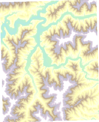
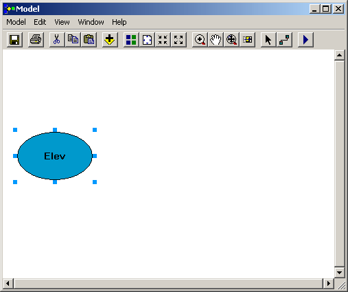
The map
contains an elevation raster for
Step 2 Enable the Spatial Analyst
extension
If you
need to load the ArcGIS Spatial Analyst extension continue with this step.
Otherwise, skip to Step 3.
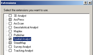
To add the
ArcGIS Spatial Analyst extension, from the Tools menu, choose Extensions. When
the Extensions dialog appears, check the Spatial Analyst box.
Note: Your list of extensions may differ from those shown in the View
Result graphic below.
Step 2: Enable the Spatial Analyst
extension.
Close the
Extensions dialog.
Step 3 Open ArcToolbox
and explore toolbox organization
If
necessary, click the Show/Hide ArcToolbox Window
button ![]() to display ArcToolbox.
to display ArcToolbox.
Step 3a: Open ArcToolbox
and explore toolbox organization.
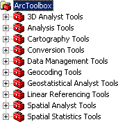
The ArcToolbox window can be docked anywhere in ArcMap, or be a
free-standing window.
The toolboxes
that are available to you are listed on the Favorites tab. The contents of this
list depend on which ArcGIS software product (ArcView,
ArcEditor, or ArcInfo) you
are using, and which extensions you have installed.
Click the
plus sign (+) to the left of the Spatial Analyst Tools toolbox to expand its
contents.
Step 3b: Open ArcToolbox
and explore toolbox organization.
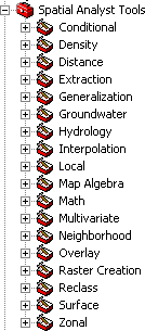
All of the
Spatial Analyst tools that come with ArcGIS have been grouped into many
different toolsets. Within each toolset, an operation is represented as a tool.
Expand the
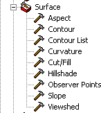
Surface toolset.
Step 3c: Open ArcToolbox
and explore toolbox organization
This
toolset contains nine tools used for analyzing surfaces. Each tool runs a
single operation on your data.
Step 4 Set the geoprocessing
environment
Before you
use a tool, you should set the appropriate geoprocessing
environment.
Right-click an empty space in ArcToolbox and
click Environments.
The geoprocessing framework has more environments than does the
Spatial Analyst toolbar because it also includes those used for vector
processing. The environments you set here are used by all geoprocessing
tools, whether you run them in ArcToolbox, the
Command Line, within ModelBuilder, or in a script.
The dialog organizes the environments under headings, like General Settings.
In the
Environment Settings dialog, click General Settings to expand it.
For
Current Workspace, click the Browse button and navigate to your Lab10a
folder.
Click the Harlan.mdb
geodatabase and click Add.
By default,
inputs and outputs are directed to your current workspace, but you can redirect
the output to another workspace or designate a default scratch workspace for
output data.
For
Scratch Workspace, click the Browse button and navigate to your Lab10a folder.
Click HarlanScratch.mdb
and click Add.
If
necessary, scroll down in the dialog, then for Output Extent, click the
dropdown arrow and choose Same as Layer "Elev" from the dropdown list.
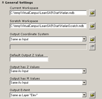
Step 4a: Set the geoprocessing environment.
Now, any geoprocessing tools that you launch from ArcToolbox will be expecting input data from the Harlan geodatabase, and all automatically generated output data will
be directed to the HarlanScratch geodatabase,
which you'll use to store all your temporary and intermediate data. You always
have the option of changing default tool parameters, of course, and you can
change your ArcToolbox environment settings at any time.
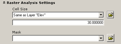
Scroll
down and click Raster Analysis Settings to expand it.
For Cell
Size, choose Same as Layer "Elev".
Step 4b: Set the geoprocessing environment.
Click OK
to close the Environment Settings dialog.
Tip: Right-clicking an empty space in ArcToolbox
and choosing Environments isn't the only way to access the Environment Settings
dialog. You can also access it from the Tools menu under Options or by clicking
the Environments button on geoprocessing tool dialogs
you open from ArcToolbox.
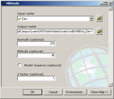
Step 5 Run a Spatial Analyst tool from its
dialog
In this
step, you'll run the Hillshade tool in the Surface
toolset.
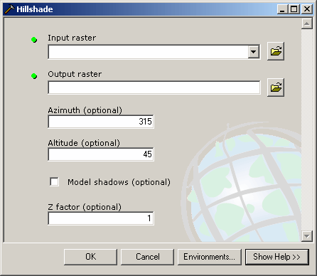
In ArcToolbox, double-click the Hillshade
tool to open its dialog.
Step 5a: Run a Spatial Analyst tool
from its dialog.
Note: You can resize the dialog for any tool. In the View Result
graphic above, the dialog has been resized to be smaller than the default
dialog size.
The dialog
contains five elements that are called parameters. Each tool parameter consists
of one or more text boxes for user input. Values set for parameters define a
tool's behavior during run time.
Two of the
parameters are marked with a green dot. The green dot indicates a required
parameter that you must fill in for the tool to run. Tool dialogs have a help
area that describes a parameter when you click its control. Also, you can use
the dialog to open the ArcGIS Desktop Help for the tool.
In the Hillshade dialog, if necessary, click Show Help, then click
Help to open the ArcGIS Desktop Help.
Briefly
review the Hillshade help; then close the ArcGIS
Desktop Help window and, if you like, click Hide Help.
Under
Input Raster, click the dropdown arrow and choose Elev
from the dropdown list.
Step 5b: Run a Spatial Analyst tool
from its dialog.
Notice
that the dialog automatically created a name for your output raster, and that
it used the path you had set for the Scratch Workspace environment.
Tip: Everytime you run a tool,
ArcMap will automatically create a default name for the layer your process will
create. While you can change this name in the Table of Contents after it has
been created, you can also change it in the dialog. To do so, scroll to the end
of the path, highlight just that portion of the path you want to change (the
layer name at the end), and type a new layer name.
All of the
required parameter values have been filled in. A tool and its parameter values is called a process. Now that the process has been defined,
you can run the tool.
Click OK
to run the Hillshade tool.
The Hillshade progress window shows the status of the
processing. When the process is complete, the new raster is added to the
display. Once the process is complete, close the status
dialog.
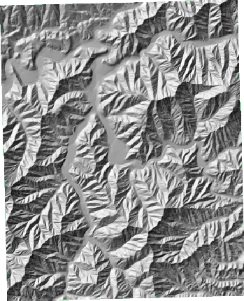
Step 5c: Run a Spatial Analyst tool
from its dialog.
You've
successfully run a Spatial Analyst tool from the tool's dialog.
Step 6 Run a Spatial Analyst tool using
the command line
In this
step, you'll use the Command Line window to run a Spatial Analyst tool and to
explore some of its capabilities. Each geoprocessing
tool in ArcToolbox has a corresponding command, which
is what you use when you write scripts. Models and scripts that you add to ArcToolbox can be run as commands as well.
Click the
Show/Hide Command Line Window button ![]() to display the Command Line window.
to display the Command Line window.
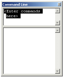
Step 6a: Run a Spatial Analyst tool
using the command line.
The top part
of the Command Line window is the command line. The bottom part is the message
area, where messages are displayed when a tool is run.
Like the ArcToolbox window, the Command Line window can be docked or
be a free-standing window. You might prefer docking the window to the bottom of
the ArcMap window. You can also resize the command and message areas.
Step 6b: Run a Spatial Analyst tool
using the command line.
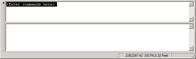
To run a
tool in the command line, you'll type the tool name followed by a series of
parameter values.
In the
command line, start typing the word Slope.
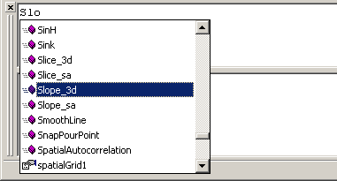
Step 6c: Run a Spatial Analyst tool
using the command line.
A list of
possible commands displays.
Note: The list displays all tools that are on the Favorites tab of ArcToolbox. (Only tools that are in ArcToolbox
can be run from the command line.)
Double-click
Slope_sa and press the space bar on your keyboard to
insert the Slope_sa tool followed by a space in the
command line.
Step 6d: Run a Spatial Analyst tool
using the command line.
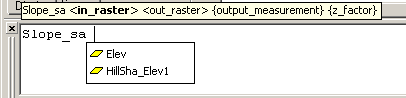
After the
tool is inserted and the space bar is pressed, usage displays above the command
line, which contains command line syntax for the tool. The usage helps you
supply parameter values in the correct manner. Required parameters appear
between the <> symbols, while optional parameters appear between the {}
symbols. These are the same parameters that you saw when you ran the Hillshade tool using a tool dialog.
You want
to calculate slope for the Elevation raster, so you'll choose Elevation as your
first parameter value. You could type the filename in the command line, or you
could drag and drop the feature class. You'll do the latter.
In the
Table of Contents, drag the Elevation raster and drop it in the command line.
Press the spacebar to see the next parameter.
Step 6e: Run a Spatial Analyst tool
using the command line.
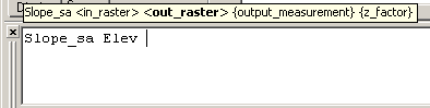
The next
required parameter is highlighted in the usage. Type SlpDeg
and press the space bar.
Step 6f: Run a Spatial Analyst tool
using the command line.
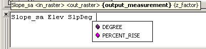
The next
parameter is optional and is highlighted in the usage. You want to calculate
slope in degrees so double-click DEGREE to add it to the command line.
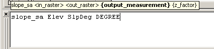
Step 6g: Run a Spatial Analyst tool
using the command line.
All of the
necessary parameters have been set, so the tool is ready to run.
Tip: An explanation of command line syntax is available in the help
document for each tool, accessible by right-clicking the tool in ArcToolbox and choosing Help.
With your
cursor still in the command line, press Enter to run the tool.
As the
tool runs, processing messages are displayed in the bottom part of the Command
Line window. These messages include such information as when the tool began
executing, which parameter values are being used, and the progress of the
tool's execution. Warnings of potential problems or errors can also be
displayed here.
You may
need to resize the window to see all of the messages.
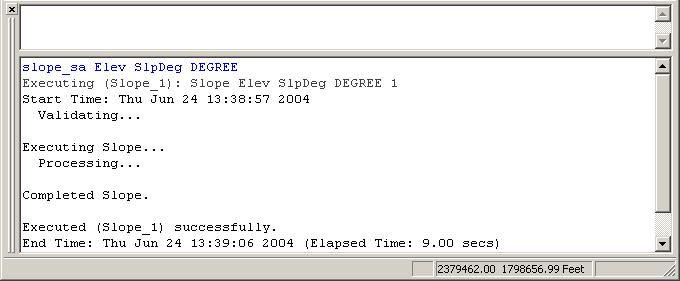
Step 6h: Run a Spatial Analyst tool
using the command line.
Step 7 Run the tool again
Once
you've run a tool in the command line, you can quickly run that tool again,
modifying any parameters as necessary.
In the
message area of the Command Line window, the tool you just ran and its
parameters are displayed in blue text.
Right-click
anywhere in the blue text and choose Recall. The tool and parameters are added
to the command line.
Before you
run the tool again, you'll change the output feature class name and the output
measurement.
In the
command line, replace SlpDeg with SlpPer.
Then replace DEGREE with PERCENT_RISE.
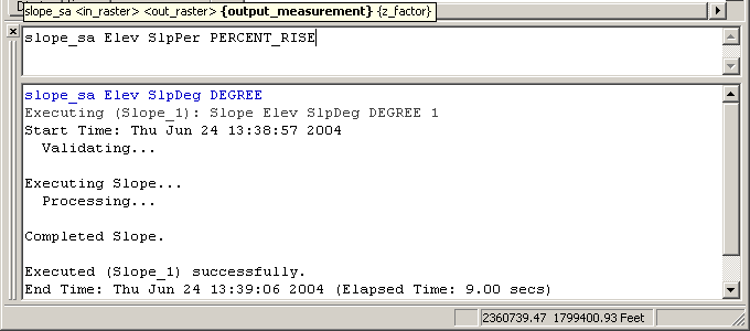
Step 7: Run the tool again.
Press
Enter to run the tool.
Until you
close ArcMap, any tool that you run, along with its parameters, will be listed
in the message area, and can be recalled to the command line. After the
application is closed, the processes are logged to a history model in the
History toolbox.
When the process is complete, close the Command Line window.
Step 8 Run Spatial Analyst tools in ModelBuilder
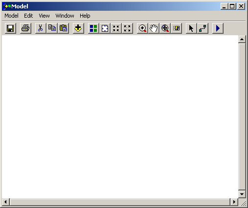
In this
step, you'll use ModelBuilder to create and run a
simple model containing several Spatial Analyst tools. Models are especially
useful for designing and running complex series of geoprocessing
tasks without the need for performing any programming.
Before you
can create a model, you'll need a toolbox or toolset to store it in as you
cannot modify the standard toolboxes.
Right-click
an empty area of ArcToolbox and choose Add Toolbox.
In the Add
Toolbox dialog, navigate to your Lab10a\Tools folder, choose HarlanTools, and click Open.
The new
toolbox is added to ArcToolbox.
Right-click
the HarlanTools toolbox, click
New, then choose Model. The ModelBuilder window
appears.
Step 8a: Run Spatial Analyst tools
in ModelBuilder.
You build
a model by dragging data from ArcMap (or ArcCatalog)
and tools from ArcToolbox into the ModelBuilder window.
From the
ArcMap Table of Contents, drag and drop the Elev
layer into the Model window.
Step 8b: Run Spatial Analyst tools
in ModelBuilder.
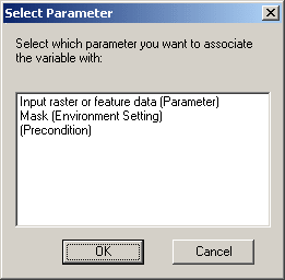
You will
be prompted to select what parameter of the file you want to work with:
Step 8c: Run Spatial Analyst tools
in ModelBuilder
Select the
Input raster or feature data[Parameter]. Then, hit OK.
From ArcToolBox, drag the Aspect, Hillshade,
and Slope tools into the model.
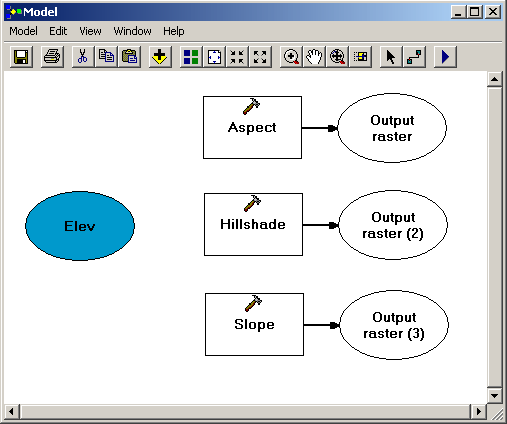
Step 8d: Run Spatial Analyst tools
in ModelBuilder.
Model
elements appear unshaded until they have enough
information to run. The tools in your model will be shaded after you connect
them to the input elevation dataset.
In the
Model window, click the Add Connection button ![]() .
.
In the
model, click the Elev dataset and drag a line to the
Aspect tool.
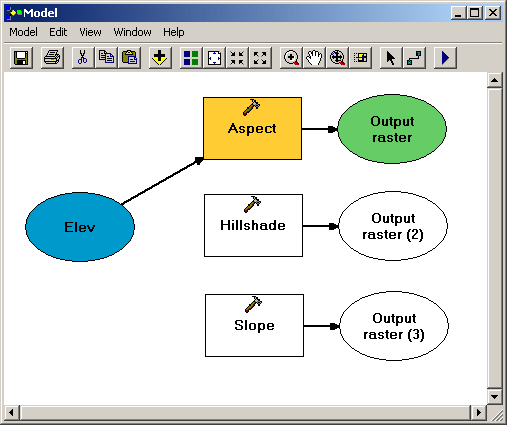
Step 8e: Run Spatial Analyst tools
in ModelBuilder.
The
connected elements are now shaded and ready to run.
Now repeat
this procedure to connect the Elev dataset to the Hillshade tool, and then again to connect it to the Slope
tool.
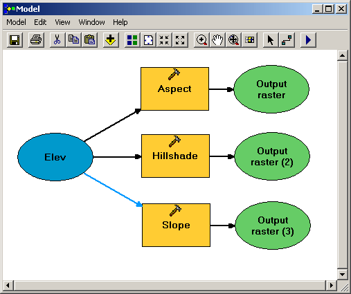
Step 8f: Run Spatial Analyst tools
in ModelBuilder.
All model
elements have context menus that appear when you right-click them. You will now
use the context menus to rename each of the output dataset elements.
Right-click
the Aspect output (Output Raster) and choose Rename to
display the Rename dialog. Replace the name Output Raster with Output Aspect.
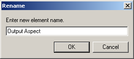
Step 8g: Run Spatial Analyst tools
in ModelBuilder.
Click OK.
Rename the
other two outputs Output Hillshade and Output
Slope.
Step 8h: Run Spatial Analyst tools
in ModelBuilder.
Click the
Auto layout button ![]() to automatically arrange the model, then, if
necessary, enlarge the Model window.
to automatically arrange the model, then, if
necessary, enlarge the Model window.
You can
run a model from a dialog, the command line, or from the ModelBuilder
window. You'll run it from ModelBuilder.
On the ModelBuilder toolbar, click the Run button
![]() .
.
Notice
that as the model runs, the tool being executed is shown in red. The progress
window tracks the progress of the geoprocessing
operations. If the Command Line window is still open, you will see that the
same information is displayed in the bottom part of that window.
When the
model finishes running, close the progress window, if necessary.
Note: Even if you selected the option to automatically close the
progress window when you ran a tool from a dialog, you have to select the
option again for the model progress window.
Notice
that the tools and the output data elements now have drop shadows. The drop
shadows indicate that the model has been run.
If you
would like to view the model results, right-click each of the output elements
in the model and choose Add to Display to add the layer to ArcMap.
When you
are finished, from the Model menu, choose Close. Click Yes
to save the changes to the model.
Step 9 Save the map document
Save the
map document as Framework2.mxd in your module folder.
You can
run any Spatial Analyst tool from either a dialog or the command line. You can
join processes together using models or scripts. While models and scripts
contain individual geoprocessing tools, they are also
considered tools themselves. A model can also be run in ModelBuilder.
All tools work essentially the same way regardless of which method you choose
to run them.
Air
ambulance study
For this
exercise, imagine that the dispatch managers of local hospitals providing air
ambulance service are working together with local schools and colleges to
conduct a preliminary study of air rescue and air ambulance service in the
As one of
the lead GIS analysts on the team, you need to determine the distance from the
schools to the hospitals, which hospitals are nearest to the schools, and the
direction from the hospitals to the schools, in order to help dispatchers
accurately determine estimated times of arrival and improve the efficiency of
the service.
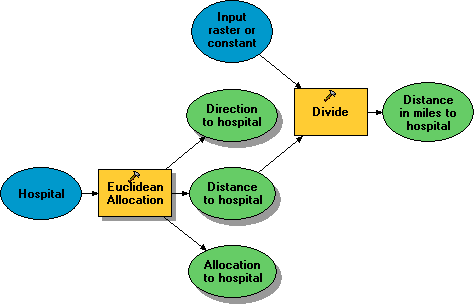
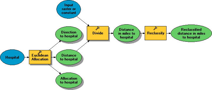
You'll
build a model that uses the Euclidean Allocation tool to create surfaces of
straight-line distance, direction, and allocation. You'll use the distance
surface to find the distance from the schools (locations on the surface) to the
nearest hospitals (source). Next, you'll explore the direction and allocation
surfaces. Finally, you'll use Map Algebra and the CON function to create a
reverse direction surface of the Direction to Hospital layer. This way,
dispatchers can also help the pilots navigate back to the hospital.
Since helicopters can fly "as the crow flies", you can
provide directions in degrees azimuth.
Estimated
time to complete: 30 minutes
Step 1 Open the map document
Start
ArcMap™ and open the Distance.mxd map document
from your Lab10a folder.
Step 1: Open the map document.
The
locations of 14 hospitals in the
If
necessary, load the ArcGIS Spatial Analyst extension and make the ArcToolbox™ window visible.
The
environment settings for this exercise have been set as follows:
General
Settings
- Current Workspace: ...\LLab10a\SanDiego.mdb
- Scratch Workspace: ...\LLab10a\SanDiegoScratch
- Output Extent: Same as Layer "Study Area"
- Output Coordinate System: Same as Layer "Study
Area"
Raster Analysis
Settings
- Cell Size: 100
- Mask: ...\SanDiego.mdb\SDCityClip
Step 2 Create an empty model
In this
step, you'll create a new model in which to perform your analysis.
Right-click
an empty area of ArcToolbox and choose Add Toolbox.
In the Add Toolbox dialog, navigate to your Lab10a\Tools folder, click DistanceTools, and click Open.
In ArcToolbox, right-click the new DistanceTools
toolbox, point to New, and choose Model to open the ModelBuilder
window.
From the
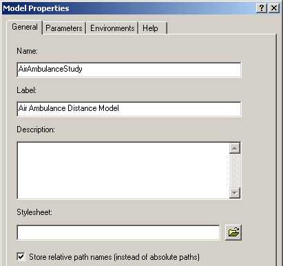
Model menu, choose Model Properties. Make sure the General tab is active.
For Name,
type AirAmbulanceStudy.
For Label,
type Air Ambulance Distance Model.
The name
defines how the tool will be referenced at the command line and in scripts.
Names do not allow spaces or certain characters such as periods because they
are not allowed in scripts. Labels determine how the model will appear in a
toolbox. You can use spaces and periods in labels to provide a clear
explanation of what the model is for.
Check the
box to store relative path names.
Step 2: Create an empty model.
Click OK.
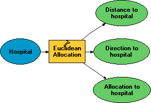
Step 3 Run the Euclidean Allocation tool
In this
step, you will use the Euclidean Allocation tool to create three new surfaces.
Surfaces created using the Euclidean Allocation tool use straight-line
(Euclidean) distance measurements. The source features in this exercise are
hospitals with air ambulance service.
Regardless
of where the school or college is located, you can use these surfaces to find
out which of the hospitals is nearest to the school, how far away the closest
hospital is from the school, and in which direction the hospital is from the
nearest school.
If
necessary, expand the Spatial Analyst toolbox. Expand the Distance toolset then
drag the Euclidean Allocation tool from ArcToolbox
into the model.
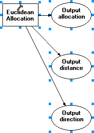
Step 3a: Run the Euclidean
Allocation tool.
In the
model, double-click the Euclidean Allocation tool.
The dialog
that opens is the same dialog that you would see if you opened the Euclidean
Allocation tool from ArcToolbox. Fill out its
parameters as follows:
Input
raster or feature source data: Hospital
Source field: ID
Output allocation raster: ...\SanDiegoScratch\EucAllocation.
Output distance raster: ...\SanDiegoScratch\EucDistance
Output direction raster: ...\SanDiegoScratch\EucDirection
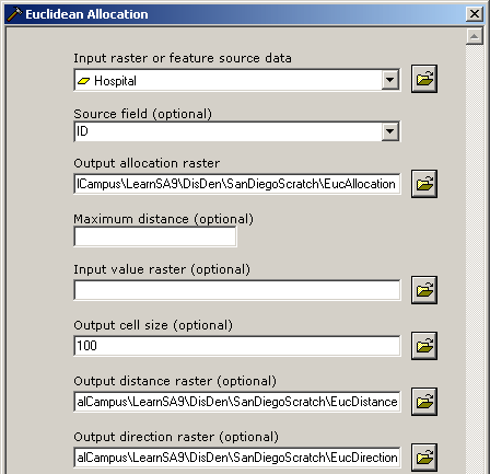
Click OK.
Tip: You can use the Auto Layout button ![]() to arrange the model after adding each new
process.
to arrange the model after adding each new
process.
Step 3c: Run the Euclidean
Allocation tool.
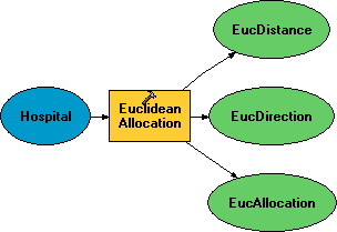
In the
model the Euclidean Allocation process is now colored in and in the "ready
to run" state.
You can
rename the output elements to assign friendlier, more helpful names. This will
not change the name on disk, but only how the element is represented in the
model and in dialogs.
Right-click
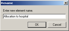
the EucAllocation element and click Rename.
In the
Rename dialog, type Allocation to hospital.
Step 3d: Run the Euclidean Allocation
tool.
Click OK.
Likewise,
rename the EucDistance and EucDirection
elements to Distance to hospital and Direction to hospital respectively.
Step 3e: Run the Euclidean
Allocation tool
In the
model, right-click Euclidean Allocation and choose Run.
Note: Choosing run for a particular tool will only execute that single
process. You will run the entire model later in this exercise.
Step 3f: Run the Euclidean
Allocation tool.
When the
process is complete, the EucAllocation, EucDistance, and EucDirection rasters are created. Notice that all of the elements have dropshadows behind them indicating that the process has
been executed.
Step 4 Investigate the Distance to
hospital surface
Once a
process has been run, you can add the results to ArcMap.
Right-click
the Distance to hospital element and choose Add to Display.
When the EucDistance layer is added to your map, move it down in the
Table of Contents so it appears just above San Diego Area.
Every cell
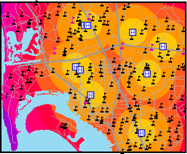
value in the Distance to hospital surface represents the straight line distance
back to the nearest hospital.
Step 4a: Investigate the Distance
to hospital surface.
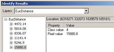
![]() 1 The
Euclidean distance function determines distance values using the same unit of
measure as the map units. In this map, which unit of measure
do the distance values use?
1 The
Euclidean distance function determines distance values using the same unit of
measure as the map units. In this map, which unit of measure
do the distance values use?
Click the
Identify button ![]() on the Tools toolbar, then click somewhere on
the map.
on the Tools toolbar, then click somewhere on
the map.
In the
Identify Results dialog, from the Layers dropdown menu, choose EucDistance.
Hold the
Shift key down and click several places on the map. You may have to move the
Identify Results dialog aside so you can see the map. The View Result graphic
below shows examples of the values you might see.
Step 4b: Investigate the Distance
to hospital surface.
![]() 2 The
Euclidean Distance function produces a raster, or in this case, a set of rasters. Which type of data are
the rasters?
2 The
Euclidean Distance function produces a raster, or in this case, a set of rasters. Which type of data are
the rasters?
Step 5 Convert distance to miles
It would
be helpful to have the distance reported in some other unit of measure, by mile
for example, but the Distance to hospital layer is a continuous surface, and
you can’t edit the attribute table.
You could,
however, convert the raster to a discrete or integer raster. You would then be
able to edit the attribute table and convert the units by adding a field to the
attribute table, calculating the values, and then converting feet to miles.
In this
exercise, however, you will create a new surface that uses a different unit of
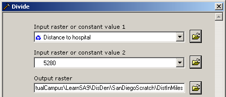
measure by using the Divide tool. Since one mile equals 5,280 feet, dividing
the raster by 5280 will create a new surface with cell values expressed in
miles.
From
within the Math toolset, drag the Divide tool into the model.
In the
model, double-click the Divide tool and fill out its parameters as follows:
Input
raster or constant value 1: Distance to hospital
Input raster or constant value 2: 5280
Output raster: ...\SanDiegoScratch\DistInMiles
Step 5a: Convert distance to miles.
Click OK.
Rename the
output element Distance in miles to hospital.
Step 5b: Convert distance to miles
In the
model, right-click the Divide tool element and choose Run.
When the process is complete, right-click the Distance in miles to hospital
element and choose Add to Display.
Move the DistInMiles raster just above EucDistance
in the Table of Contents.
Step 5c: Convert distance to miles.
Use the
Identify tool ![]() to query cell values for the new surface. The
new layer is still a continuous surface, but the cell values are now expressed
in miles.
to query cell values for the new surface. The
new layer is still a continuous surface, but the cell values are now expressed
in miles.
Step 6 Reclassify the Distance in miles to
hospital layer
Reclassifying
the Distance in miles to hospital layer will allow dispatchers to visually
assess the approximate distances to schools in easier-to-read zones. For
example, the dispatcher could look at the map and quickly determine that a
particular school is about 4 miles from the nearest hospital. The exact
distance values are still contained in the Distance in miles to hospital
surface.
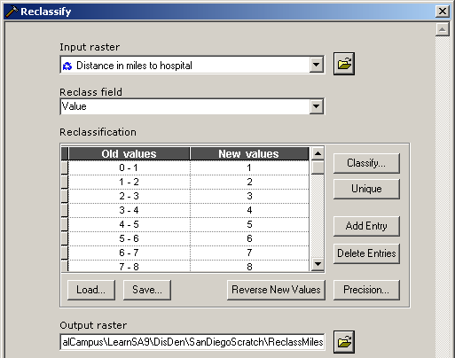
From
within the Reclass toolset, drag the Reclassify tool
into the model.
In the
model, double-click the Reclassify tool and fill out its parameters as follows:
Input
raster: Distance in miles to hospital
Reclass field: Value
Click
Classify.
For
Method, choose Defined Interval.
For
Interval Size, change the value to 1 and press your Tab key.
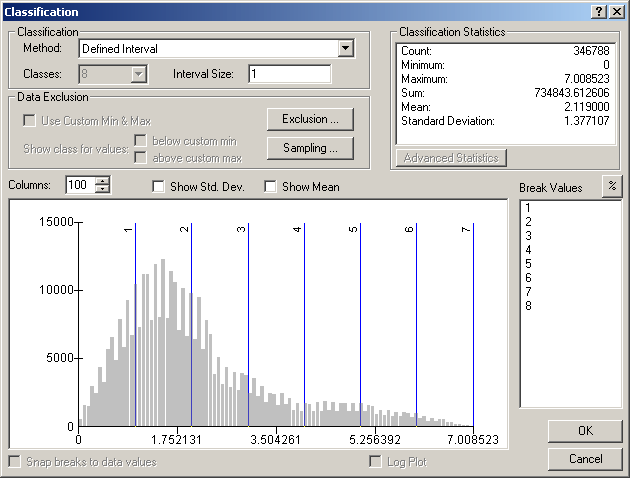
Step 6a: Reclassify the Distance in
miles to hospital layer.
Click OK.
For Output
raster, maintain the default workspace folder, but change the raster name to ReclassMiles.
Step 6b: Reclassify the Distance in
miles to hospital layer.
Click OK.
Rename the
output element Reclassified distance in miles to hospital.
Step 6c: Reclassify the Distance in
miles to hospital layer
In the
model, right-click the Reclassify tool element and choose Run.
When the process is complete, right-click the Reclassified distance in miles
to hospital element and choose Add to Display.
Move the ReclassMiles raster just above DistInMiles
in the Table of Contents.
In the
Table of Contents, double-click the ReclassMiles
layer to open its Layer Properties dialog then click the Symbology
tab.
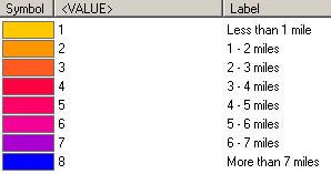
Symbolize ReclassMiles using 8 unique values and apply the Distance
color scheme.
![]()
Change the
Label text for the symbols to match the following table.
|
Value |
Label |
|
1 |
Less
than 1 mile |
|
2 |
1 - 2
miles |
|
3 |
2 - 3
miles |
|
4 |
3 - 4
miles |
|
5 |
4 - 5
miles |
|
6 |
5 - 6
miles |
|
7 |
6 - 7
miles |
|
8 |
More
than 7 miles |
Step 6d: Reclassify the Distance in
miles to hospital layer.
Click OK
to close the Layer Properties dialog.
Step 6e: Reclassify the Distance in
miles to hospital layer.
Now a
dispatcher can quickly estimate the distance to any school by simply selecting
a school and looking at the map. Clicking on the Distance in miles to hospital
layer at a school location with the Identify tool will provide a more accurate
distance to nearest hospital report.
Look at
the map and try to estimate the distance from a school to the nearest hospital,
then use the Identify tool to see how close your estimate was.
Hint: Click on the school with the Reclassified distance in miles to
hospital layer entered in the Identify Results dialog.
Close the
Identify Results dialog when you are finished.
![]() 3 When
you classify a raster layer, you're symbolizing the existing data to make it
more understandable. What happens when you reclassify a raster layer?
3 When
you classify a raster layer, you're symbolizing the existing data to make it
more understandable. What happens when you reclassify a raster layer?
The same thing as when you classify the raster
layer
The cell values in the existing raster layer are replaced by new
values that you have specified
Reclassification only works on discrete data
A new raster layer is created, where the old cell values are
replaced by new values that you have specified
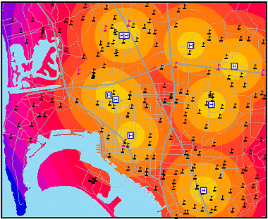
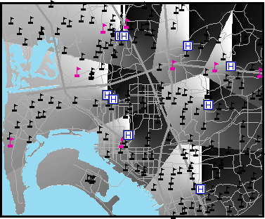
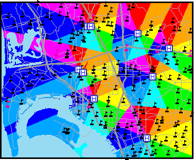
Step 7 Explore the Allocation to Hospital
layer
One output
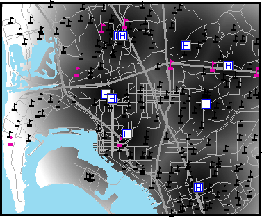
of the Euclidean Allocation tool is an allocation layer. Allocation simply
means certain cells are assigned to certain sources. In this case, cells are
assigned to the nearest hospital. Because the allocation is based on straight
line distance, the allocated cells form zones around the hospital locations.
In the
model, right-click the Allocation to hospital element and choose Add to
Display.
Move the EucAllocation raster just above ReclassMiles
in the Table of Contents.
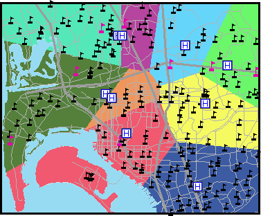
Step 7: Explore the Allocation to
Hospital layer.
The
allocation zones are composed of cells with like values. If you were to use the
Identify tool to query the surface, you would find that the cell values range
from 1 to 9, so there is a number for each hospital.
![]() 4 You
can use the Identify tool to query the EucAllocation
(Allocation to hospital) layer to find out the cell value used for each
allocation zone. Which of the following is not a way to find the range of cell
values?
4 You
can use the Identify tool to query the EucAllocation
(Allocation to hospital) layer to find out the cell value used for each
allocation zone. Which of the following is not a way to find the range of cell
values?
Look in the Layer Properties dialog, on the
Source tab in the statistics area
Examine the Value field in the Attributes of Allocation to
hospital table
Look in the Table of Contents, at the
Allocation to hospital layer symbology
Look in the Data Frame Properties dialog, on the General tab in
the Units area
Later in
the study, it might be useful to convert the Allocation to Hospital layer from
raster to vector and perform an overlay analysis of the schools and colleges to
find out how many of each exist per zone.
For now, turn
off the Allocation to Hospital layer.
Step 8 Explore the Direction to Hospital
layer
In the
model, right-click the Direction to hospital element and choose Add to Display.
Move the EucDirection raster just above EucAllocation
in the Table of Contents.
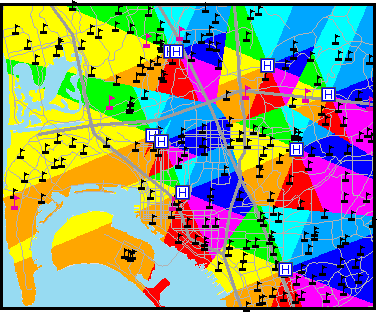
Step 8a: Explore the Direction to
Hospital layer.
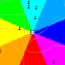
When this
layer was created, it was based on the hospital locations, giving each cell a
value that indicates the direction to the nearest hospital along a straight
line. The direction value is expressed in degrees. Cells in the direction
surface that correspond to source locations (i.e., hospitals) have a value of
zero, or no direction.
Another
way to think about the direction surface values is to imagine a compass circle
around any cell location on the map.
At the top of the circle is north. If you centered the compass circle on a school location, the Direction to hospital cell value that corresponds with that location would be the direction to the nearest hospital.
Explore
the EucDirection surface using the Identify tool.
First,
zoom in to one of the hospitals so that you can see several of the school
locations surrounding it. Center the hospital in your display.
Step 8b: Explore the Direction to
Hospital layer.
Select the
Identify tool and click somewhere on the map. Move the Identify Results dialog
so you can see the map.
In the
Identify Results dialog, click the Layers dropdown arrow and choose EucDirection.
Now click
a school location on the map.
The
direction back to the nearest hospital is reported.
![]() 5 The
cell values of a Euclidean (straight-line) direction surface indicate the direction
back to the nearest source location in degrees azimuth no matter how far the
cell is from the nearest source.
5 The
cell values of a Euclidean (straight-line) direction surface indicate the direction
back to the nearest source location in degrees azimuth no matter how far the
cell is from the nearest source.
True
False
Try
clicking more places on the map. Notice distance from the hospital does not
affect direction, and if you click on the exact location of the hospital, the
direction value is zero.
When you
are finished, click the Full Extent button.
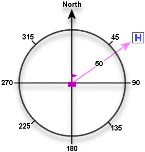
Step 9 Consider creating a reverse
direction surface
The
Direction to hospital surface helps air ambulance dispatchers direct pilots at
a location back to the nearest hospital. Dispatchers, however, must first
direct the pilots from the hospital to the location.
So, now
you need a surface where the imaginary compass is centered on the hospitals, as
shown here.
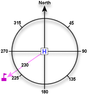
To do this you will create a new surface where all of the current values in the Direction to hospital surface point in the exact opposite direction (180 degrees).
First,
however, consider the problem:
- Each new cell value for the
reverse direction surface must be plus or minus 180 degrees from the
Direction to hospital surface values.
- The reverse direction surface
cannot have values over 360 degrees.
- Adding 180 to values less than
or equal to 180, and subtracting 180 to values greater than 180, would
work, except for one problem: the zero values. You need to maintain the
zero values in the direction surface because they represent the source
locations.
Using the
CON function in the Map Algebra expression will maintain the zero values of the
source locations.
Step 10 Use the CON function to create a
reverse direction surface
In this step,
you will use the CON function to create a reverse direction surface from the
existing Direction to hospital surface.
First, you
will build an expression to visualize the logic of the conditional statement
and pre-determine if you would get the results you need if you were to use it.
After examining the first expression, you will refine it by embedding another
CON function within the first CON function. You will then use this expression
to create a new surface from the Direction to Hospital layer.
From the
Map Algebra toolset, drag the Single Output Map Algebra tool into the model.
In the
model, double-click the Single Output Map Algebra tool and fill out its
parameters as follows:
con([Direction
to hospital] > 0 & [Direction to hospital] <= 180,[Direction to
hospital] + 180,[Direction to hospital] - 180)
For Output
raster, maintain the default workspace folder, but change the raster name to RevDir.
For Input
raster or feature data to show in ModelBuilder,
select Direction to hospital from the dropdown list.
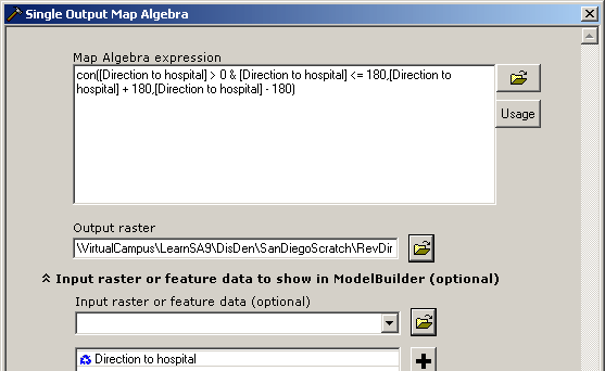
Step 10a: Use the CON function to
create a reverse direction surface.
Don't
click OK just yet.
If you were
to run this tool, a new surface would be created following an IF, THEN, ELSE
form of evaluation of the Direction to hospital surface. In other words, the
surface would be created based on the statement: IF the cell values in the
Direction to hospital surface are greater than zero, but less than or equal to
180, THEN add 180 to each cell value. Or ELSE, subtract 180 from each cell
value.
Although
this expression could be run successfully, the zero values, or source cells,
would end up with a value of -180.
To
maintain the zero values, you will use a different conditional statement, one
that embeds the CON function within the existing CON function.
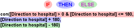
Within the
statement you just created, embed another CON function statement for the ELSE
portion of the expression.
con([Direction
to hospital] > 0 & [Direction to hospital] <= 180,[Direction to
hospital] + 180,con([Direction to hospital] > 180, [Direction to hospital]
- 180,0))
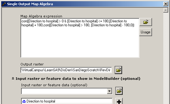
Step 10b: Use the CON function to
create a reverse direction surface.
In this
expression: IF the cell values in the Direction to hospital surface are greater
than zero, but less than or equal to 180, THEN add 180 to each cell value.
Otherwise, if cell values are greater than 180, subtract 180 from each cell
value. But, if cell values do not match any of these criteria, give them a
value of zero. Notice the two parentheses at the end of the expression. The
inside parenthesis belongs to the embedded CON function and the outside
parenthesis belongs to the first CON function.
Now click
OK.
Rename the
output element Direction from hospital.
Step 10c: Use the CON function to
create a reverse direction surface.
In the
model, right-click the Single Output Map Algebra tool element and choose Run.
When the process is complete, right-click the Direction from hospital
element and choose Add to Display.
Move the RevDir raster just above EucDirection
in the Table of Contents.
Step 10d: Use the CON function to
create a reverse direction surface.
To compare
the RevDir raster to the EucDirection
raster, you can symbolize it to use the same color scheme.
Right-click
the EucDirection layer in the Table of Contents and
choose Save as Layer file. Navigate to your Lab10a folder and save the file as EucDirection.lyr.
Now in the
Table of Contents, double-click the RevDir layer to
open its Layer Properties dialog.
With the Symbology tab active, in the Show pane on the left, choose
Classified then click Import. Navigate to your module folder, click EucDirection.lyr, and click Add.
Click OK
to close the Layer Properties dialog.
Step 10e: Use the CON function to
create a reverse direction surface.
Step 11 Save the map document
In the ModelBuilder window, click the Auto layout button ![]() to automatically arrange the model.
to automatically arrange the model.
From the
Model menu, choose Close. Click Yes to save the changes to the model.
Save the
map document as Distance2.mxd in your Lab10a folder.
You have
just created a simple model to improve initial response times for the local air
rescue and air ambulance services. The model created surfaces of Euclidean
allocation, direction, and distance.
Straight
Line Distance functions create continuous surfaces where a distance value is
assigned to each cell in the surface. These functions use Euclidean
measurements: the distance is measured along a straight line, from the cell
center to the nearest source. Distance units are measured in map units. If the
map units are in feet, then the distance value assigned to each cell is also in
feet.
Cell
values in a straight-line direction surface provide compass directions to the
nearest location of a source or sources. Cell values range from 0 to 360 with
north being 360. Zero values indicate no direction. Source cells or cells that
correspond to source locations have zero values in a straight-line direction
surface. You can create a straight-line direction surface when you create a
straight-line distance surface.